• Descriptive
    • Moments
    • Concentration
    • Central Tendency
    • Variability
    • Stem-and-Leaf Plot
    • Histogram & Frequency Table
    • Data Quality Forensics
    • Conditional EDA
    • Quantiles
    • Kernel Density Estimation
    • Normal QQ Plot
    • Bootstrap Plot

    • Multivariate Descriptive Statistics
  • Distributions
    • Binomial Probabilities
    • Geometric Probabilities
    • Negative Binomial Probabilities
    • Hypergeometric Probabilities
    • Multinomial Probabilities
    • Dirichlet
    • Poisson Probabilities

    • Exponential
    • Gamma
    • Erlang
    • Weibull
    • Rayleigh
    • Maxwell-Boltzmann
    • Lognormal
    • Pareto
    • Inverse Gamma
    • Inverse Chi-Square

    • Beta
    • Power
    • Beta Prime (Inv. Beta)
    • Triangular

    • Normal (area)
    • Logistic
    • Laplace
    • Cauchy (standard)
    • Cauchy (location-scale)
    • Gumbel
    • Fréchet
    • Generalized Extreme Value

    • Normal RNG
    • ML Fitting
    • Tukey Lambda PPCC
    • Box-Cox Normality Plot
    • Noncentral t
    • Noncentral F
    • Sample Correlation r

    • Empirical Tests
  • Hypotheses
    • Theoretical Aspects of Hypothesis Testing
    • Bayesian Inference
    • Minimum Sample Size

    • Empirical Tests
    • Multivariate (pair-wise) Testing
  • Models
    • Manual Model Building
    • Guided Model Building
  • Time Series
    • Time Series Plot
    • Decomposition
    • Exponential Smoothing

    • Blocked Bootstrap Plot
    • Mean Plot
    • (P)ACF
    • VRM
    • Standard Deviation-Mean Plot
    • Spectral Analysis
    • ARIMA

    • Cross Correlation Function
    • Granger Causality
  1. Probability Distributions
  2. 12  Bernoulli Distribution
  • Preface
  • Getting Started
    • 1  Introduction
    • 2  Why Do We Need Innovative Technology?
    • 3  Basic Definitions
    • 4  The Big Picture: Why We Analyze Data
  • Introduction to Probability
    • 5  Definitions of Probability
    • 6  Jeffreys’ axiom system
    • 7  Bayes’ Theorem
    • 8  Sensitivity and Specificity
    • 9  Naive Bayes Classifier
    • 10  Law of Large Numbers

    • 11  Problems
  • Probability Distributions
    • 12  Bernoulli Distribution
    • 13  Binomial Distribution
    • 14  Geometric Distribution
    • 15  Negative Binomial Distribution
    • 16  Hypergeometric Distribution
    • 17  Multinomial Distribution
    • 18  Poisson Distribution

    • 19  Uniform Distribution (Rectangular Distribution)
    • 20  Normal Distribution (Gaussian Distribution)
    • 21  Gaussian Naive Bayes Classifier
    • 22  Chi Distribution
    • 23  Chi-squared Distribution (1 parameter)
    • 24  Chi-squared Distribution (2 parameters)
    • 25  Student t-Distribution
    • 26  Fisher F-Distribution
    • 27  Exponential Distribution
    • 28  Lognormal Distribution
    • 29  Gamma Distribution
    • 30  Beta Distribution
    • 31  Weibull Distribution
    • 32  Pareto Distribution
    • 33  Inverse Gamma Distribution
    • 34  Rayleigh Distribution
    • 35  Erlang Distribution
    • 36  Logistic Distribution
    • 37  Laplace Distribution
    • 38  Gumbel Distribution
    • 39  Cauchy Distribution
    • 40  Triangular Distribution
    • 41  Power Distribution
    • 42  Beta Prime Distribution
    • 43  Sample Correlation Distribution
    • 44  Dirichlet Distribution
    • 45  Generalized Extreme Value (GEV) Distribution
    • 46  Frechet Distribution
    • 47  Noncentral t Distribution
    • 48  Noncentral F Distribution
    • 49  Inverse Chi-Squared Distribution
    • 50  Maxwell-Boltzmann Distribution
    • 51  Distribution Relationship Map

    • 52  Problems
  • Descriptive Statistics & Exploratory Data Analysis
    • 53  Types of Data
    • 54  Datasheets

    • 55  Frequency Plot (Bar Plot)
    • 56  Frequency Table
    • 57  Contingency Table
    • 58  Binomial Classification Metrics
    • 59  Confusion Matrix
    • 60  ROC Analysis

    • 61  Stem-and-Leaf Plot
    • 62  Histogram
    • 63  Data Quality Forensics
    • 64  Quantiles
    • 65  Central Tendency
    • 66  Variability
    • 67  Skewness & Kurtosis
    • 68  Concentration
    • 69  Notched Boxplot
    • 70  Scatterplot
    • 71  Pearson Correlation
    • 72  Rank Correlation
    • 73  Partial Pearson Correlation
    • 74  Simple Linear Regression
    • 75  Moments
    • 76  Quantile-Quantile Plot (QQ Plot)
    • 77  Normal Probability Plot
    • 78  Probability Plot Correlation Coefficient Plot (PPCC Plot)
    • 79  Box-Cox Normality Plot
    • 80  Kernel Density Estimation
    • 81  Bivariate Kernel Density Plot
    • 82  Conditional EDA: Panel Diagnostics
    • 83  Bootstrap Plot (Central Tendency)
    • 84  Survey Scores Rank Order Comparison
    • 85  Cronbach Alpha

    • 86  Equi-distant Time Series
    • 87  Time Series Plot (Run Sequence Plot)
    • 88  Mean Plot
    • 89  Blocked Bootstrap Plot (Central Tendency)
    • 90  Standard Deviation-Mean Plot
    • 91  Variance Reduction Matrix
    • 92  (Partial) Autocorrelation Function
    • 93  Periodogram & Cumulative Periodogram

    • 94  Problems
  • Hypothesis Testing
    • 95  Normal Distributions revisited
    • 96  The Population
    • 97  The Sample
    • 98  The One-Sided Hypothesis Test
    • 99  The Two-Sided Hypothesis Test
    • 100  When to use a one-sided or two-sided test?
    • 101  What if \(\sigma\) is unknown?
    • 102  The Central Limit Theorem (revisited)
    • 103  Statistical Test of the Population Mean with known Variance
    • 104  Statistical Test of the Population Mean with unknown Variance
    • 105  Statistical Test of the Variance
    • 106  Statistical Test of the Population Proportion
    • 107  Statistical Test of the Standard Deviation \(\sigma\)
    • 108  Statistical Test of the difference between Means -- Independent/Unpaired Samples
    • 109  Statistical Test of the difference between Means -- Dependent/Paired Samples
    • 110  Statistical Test of the difference between Variances -- Independent/Unpaired Samples

    • 111  Hypothesis Testing for Research Purposes
    • 112  Decision Thresholds, Alpha, and Confidence Levels
    • 113  Bayesian Inference for Decision-Making
    • 114  One Sample t-Test
    • 115  Skewness & Kurtosis Tests
    • 116  Paired Two Sample t-Test
    • 117  Wilcoxon Signed-Rank Test
    • 118  Unpaired Two Sample t-Test
    • 119  Unpaired Two Sample Welch Test
    • 120  Two One-Sided Tests (TOST) for Equivalence
    • 121  Mann-Whitney U test (Wilcoxon Rank-Sum Test)
    • 122  Bayesian Two Sample Test
    • 123  Median Test based on Notched Boxplots
    • 124  Chi-Squared Tests for Count Data
    • 125  Kolmogorov-Smirnov Test
    • 126  One Way Analysis of Variance (1-way ANOVA)
    • 127  Kruskal-Wallis Test
    • 128  Two Way Analysis of Variance (2-way ANOVA)
    • 129  Repeated Measures ANOVA
    • 130  Friedman Test
    • 131  Testing Correlations
    • 132  A Note on Causality

    • 133  Problems
  • Regression Models
    • 134  Simple Linear Regression Model (SLRM)
    • 135  Multiple Linear Regression Model (MLRM)
    • 136  Logistic Regression
    • 137  Generalized Linear Models
    • 138  Multinomial and Ordinal Logistic Regression
    • 139  Cox Proportional Hazards Regression
    • 140  Conditional Inference Trees
    • 141  Leaf Diagnostics for Conditional Inference Trees
    • 142  Conditional Random Forests
    • 143  Hypothesis Testing with Linear Regression Models (from a Practical Point of View)

    • 144  Problems
  • Introduction to Time Series Analysis
    • 145  Case: the Market of Health and Personal Care Products
    • 146  Decomposition of Time Series
    • 147  Ad hoc Forecasting of Time Series
  • Box-Jenkins Analysis
    • 148  Introduction to Box-Jenkins Analysis
    • 149  Theoretical Concepts
    • 150  Stationarity
    • 151  Identifying ARMA parameters
    • 152  Estimating ARMA Parameters and Residual Diagnostics
    • 153  Forecasting with ARIMA models
    • 154  Intervention Analysis
    • 155  Cross-Correlation Function
    • 156  Transfer Function Noise Models
    • 157  General-to-Specific Modeling
  • Model Building Strategies
    • 158  Introduction to Model Building Strategies
    • 159  Manual Model Building
    • 160  Model Validation
    • 161  Regularization Methods
    • 162  Hyperparameter Optimization Strategies
    • 163  Guided Model Building in Practice
    • 164  Diagnostics, Revision, and Guided Forecasting
    • 165  Leakage, Target Encoding, and Robust Regression
  • References
  • Appendices
    • Appendices
    • A  Method Selection Guide
    • B  Presentations and Teaching Materials
    • C  R Language Concepts for Statistical Computing
    • D  Matrix Algebra
    • E  Standard Normal Table (Gaussian Table)
    • F  Critical values of Student’s \(t\) distribution with \(\nu\) degrees of freedom
    • G  Upper-tail critical values of the \(\chi^2\)-distribution with \(\nu\) degrees of freedom
    • H  Lower-tail critical values of the \(\chi^2\)-distribution with \(\nu\) degrees of freedom

Table of contents

  • 12.1 Definition
  • 12.2 Distribution Function
  • 12.3 Mean
  • 12.4 Mode
  • 12.5 Median
  • 12.6 Variance
  • 12.7 Moment Generating Function
  • 12.8 Coefficient of Skewness
  • 12.9 Coefficient of Kurtosis
  • 12.10 Parameter Estimation
  • 12.11 Purpose
  • 12.12 R Module
  • 12.13 Example
  1. Probability Distributions
  2. 12  Bernoulli Distribution

12  Bernoulli Distribution

This distribution models the simplest random experiment: exactly one trial with two possible outcomes (success/failure, yes/no, pass/fail).

12.1 Definition

The Bernoulli Distribution is named after the mathematician Jacob Bernoulli (Bernoulli 1713) and describes a binary random variable \(X\) that can only be “success” or “failure.”

\[ \text{P}(X=1)=p, \quad \text{P}(X=0)=q=1-p \]

where \(p\) = probability of success and \(q\) = probability of failure.

Equivalent PMF form:

\[ \text{P}(X=x) = p^x(1-p)^{1-x}, \quad x \in \{0,1\} \]

12.2 Distribution Function

\[ F(x)= \begin{cases} 0, & x < 0\\ q, & 0 \le x < 1\\ 1, & x \ge 1 \end{cases} \]

12.3 Mean

\[ \text{E}(X) = p \]

The mean value (or “expected” value) of the outcome \(X\) of the Bernoulli experiment is equal to the probability of obtaining a success. This result can be intuitively interpreted as the expected or average outcome of \(X\) when the Bernoulli experiment is repeated \(N\) times: the average of \(X\) becomes \(\frac{pN}{N} = p\).

12.4 Mode

\[ \begin{align*} \begin{cases}\text{Mo}(X) = 0 &\text{ if } q > p\\\text{Mo}(X) = 0,1 &\text{ if } q = p\\\text{Mo}(X) = 1 &\text{ if } q < p\end{cases} \end{align*} \]

When \(p=q=0.5\), both 0 and 1 are modes (bimodal tie).

12.5 Median

\[ \begin{align*}\begin{cases}\text{Med}(X) = 0 &\text{ if } q > p\\\text{Med}(X) \in [0,1] &\text{ if } q = p\\\text{Med}(X) = 1 &\text{ if } q < p\end{cases}\end{align*} \]

At \(p=q=0.5\), any value in \([0,1]\) is a valid median because both median inequalities are satisfied: \(\text{P}(X \le m)\ge 0.5\) and \(\text{P}(X \ge m)\ge 0.5\).

12.6 Variance

\[ \text{V}(X) = p q \]

Intuition: variability is highest when outcomes are most uncertain (\(p=q=0.5\)), and it goes to zero as \(p \to 0\) or \(p \to 1\).

12.7 Moment Generating Function

\[ M_X(t)=\text{E}(e^{tX})=q+pe^t \]

12.8 Coefficient of Skewness

\[ g_1 = \frac{q-p}{\sqrt{pq}} \]

Interpretation: \(g_1>0\) when \(p<0.5\) (right-skewed toward 1), \(g_1<0\) when \(p>0.5\) (left-skewed toward 0), and \(g_1=0\) when \(p=0.5\).

12.9 Coefficient of Kurtosis

\[ g_2 = \frac{1-3pq}{pq} \]

The corresponding excess kurtosis is \(\frac{1-6pq}{pq}\).

Interpretation: kurtosis is smallest at \(p=0.5\) (\(g_2=1\)), increases as outcomes become more imbalanced, and diverges as \(p \to 0\) or \(p \to 1\).

12.10 Parameter Estimation

For a sample \(x_1,\dots,x_n\) with \(x_i \in \{0,1\}\), the maximum-likelihood estimator is

\[ \hat p = \bar x = \frac{1}{n}\sum_{i=1}^n x_i. \]

12.11 Purpose

The Bernoulli model is the building block for many discrete models:

  • It is the one-trial version of a success/failure experiment.
  • Repeating Bernoulli trials leads to the Binomial model (see Chapter 13).
  • It is used in quality-control pass/fail checks, click/no-click events, and yes/no diagnostic outcomes.

12.12 R Module

You can compute Bernoulli probabilities in R with dbinom using size = 1:

p_demo <- 0.35

cat("PMF values at x = 0 and x = 1:\n")
print(dbinom(c(0, 1), size = 1, prob = p_demo))

cat("\nCDF value P(X <= 0):", pbinom(0, size = 1, prob = p_demo), "\n")
cat("Random Bernoulli draws (n = 10):\n")
set.seed(123)
print(rbinom(10, size = 1, prob = p_demo))
PMF values at x = 0 and x = 1:
[1] 0.65 0.35

CDF value P(X <= 0): 0.65 
Random Bernoulli draws (n = 10):
 [1] 0 1 0 1 1 0 0 1 0 0

12.13 Example

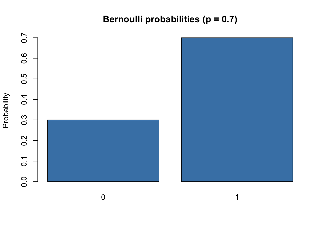
Suppose a quality-control test marks one product as either “pass” (=1) or “fail” (=0). If the pass probability is \(p = 0.7\), then:

p <- 0.7
probs <- c(`0` = 1 - p, `1` = p)
print(probs)
barplot(probs, col = "steelblue", ylab = "Probability",
        main = "Bernoulli probabilities (p = 0.7)")

  0   1 
0.3 0.7 
Bernoulli, Jacob. 1713. Ars Conjectandi. Basel: Thurnisiorum Fratrum.
Probability Distributions
13  Binomial Distribution

© 2026 Patrick Wessa. Provided as-is, without warranty.

Feedback: e-mail | Anonymous contributions: click to copy (Sats) | click to copy (XMR)

Cookie Preferences