The Beta distribution is designed for quantities bounded between zero and one: proportions, probabilities, and rates. It is the standard choice whenever a fraction or probability is itself uncertain, and it is the natural conjugate prior for Binomial data in Bayesian analysis.
Formally, the random variate \(X\) defined for the range \(0 \leq X \leq 1\), is said to have a Beta Distribution (i.e. \(X \sim \text{Beta}(\alpha, \beta)\)) with shape parameters \(\alpha > 0\) and \(\beta > 0\).
The Beta distribution is the natural choice for modelling proportions, probabilities, and rates constrained to \([0, 1]\). In R, the two shape parameters are referred to as shape1 (\(= \alpha\)) and shape2 (\(= \beta\)). The Beta distribution also serves as the conjugate prior for the Binomial and Bernoulli likelihoods in Bayesian inference (see Chapter 7 and Chapter 113).
where \(\text{B}(\alpha, \beta) = \Gamma(\alpha)\Gamma(\beta)/\Gamma(\alpha+\beta)\) is the Beta function.
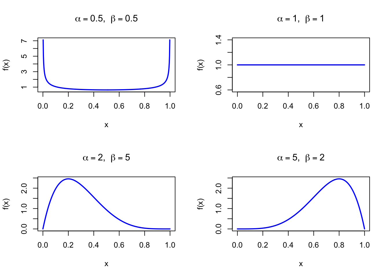
The figure below shows examples of the Beta Probability Density Function for different parameter combinations.
Code
par(mfrow =c(2, 2))x <-seq(0, 1, length =500)plot(x, dbeta(x, shape1 =0.5, shape2 =0.5), type ="l", lwd =2, col ="blue",xlab ="x", ylab ="f(x)", main =expression(paste(alpha ==0.5, ", ", beta ==0.5)))plot(x, dbeta(x, shape1 =1, shape2 =1), type ="l", lwd =2, col ="blue",xlab ="x", ylab ="f(x)", main =expression(paste(alpha ==1, ", ", beta ==1)))plot(x, dbeta(x, shape1 =2, shape2 =5), type ="l", lwd =2, col ="blue",xlab ="x", ylab ="f(x)", main =expression(paste(alpha ==2, ", ", beta ==5)))plot(x, dbeta(x, shape1 =5, shape2 =2), type ="l", lwd =2, col ="blue",xlab ="x", ylab ="f(x)", main =expression(paste(alpha ==5, ", ", beta ==2)))par(mfrow =c(1, 1))
Figure 30.1: Beta Probability Density Function for various parameter combinations
30.2 Purpose
The Beta distribution is used whenever the quantity of interest is a proportion, probability, or rate — something constrained to \([0, 1]\). Its two shape parameters allow it to take a wide variety of shapes: symmetric or skewed in either direction, bell-shaped or U-shaped, concentrated near a boundary or spread across the full interval. Common applications include:
Modelling click-through rates, conversion rates, and defect proportions
Bayesian posterior for an unknown success probability (conjugate prior for Binomial data)
Prior and posterior distributions for proportions in A/B testing
Representing subjective uncertainty about an unknown probability
Distribution of order statistics from the Uniform distribution on \([0,1]\)
Relation to the discrete setting. The Beta distribution is the continuous analog of the Binomial distribution in a precise Bayesian sense: if the unknown success probability \(p\) is given a \(\text{Beta}(\alpha, \beta)\) prior and \(k\) successes are observed in \(n\) trials, the posterior is \(\text{Beta}(\alpha + k,\, \beta + n - k)\). The Binomial models discrete counts given a fixed probability; the Beta models uncertainty about that probability itself. Beta\((\alpha, \beta)\) with positive-integer parameters is also the distribution of the \(\alpha\)-th order statistic from \((\alpha + \beta - 1)\) i.i.d. \(\text{U}(0,1)\) draws, linking it to the Uniform distribution on the discrete side.
where \(I_x(\alpha, \beta) = \text{B}(x;\, \alpha, \beta)/\text{B}(\alpha, \beta)\) is the regularized incomplete beta function. It is computed by pbeta() in R.
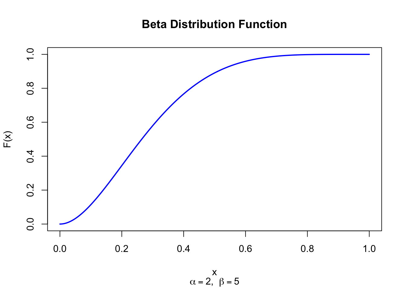
The figure below shows the Beta Distribution Function for \(\alpha = 2\) and \(\beta = 5\).
Code
x <-seq(0, 1, length =500)plot(x, pbeta(x, shape1 =2, shape2 =5), type ="l", lwd =2, col ="blue",xlab ="x", ylab ="F(x)", main ="Beta Distribution Function",sub =expression(paste(alpha ==2, ", ", beta ==5)))
Figure 30.2: Beta Distribution Function (alpha = 2, beta = 5)
30.4 Moment Generating Function
The moment generating function of the Beta distribution is expressed as a confluent hypergeometric series:
where the uncentered moments \(\mu_1', \ldots, \mu_4'\) are given by the formulas above. An equivalent expression in terms of the variance and kurtosis is \(\mu_4 = g_2 \cdot \mu_2^2\), where \(g_2\) is defined in Section Section 30.17.
The median of the Beta distribution has no general closed form. It is computed numerically in R:
# Median for Beta(2, 5)qbeta(0.5, shape1 =2, shape2 =5)
[1] 0.26445
A well-known approximation is \(\text{Med}(X) \approx (\alpha - 1/3)/(\alpha + \beta - 2/3)\) for \(\alpha, \beta > 1\), but direct computation via qbeta is preferred.
A website’s click-through rate (CTR) is modelled using Bayesian inference. We observe 5 clicks out of 50 impressions and combine this with a weak prior \(\text{Beta}(1, 1)\) (Uniform, expressing no prior knowledge). Bayesian updating with a Binomial likelihood gives the posterior:
Beta random variates can be generated from two independent Gamma variates. If \(Y_1 \sim \text{Gamma}(\alpha, 1)\) and \(Y_2 \sim \text{Gamma}(\beta, 1)\) are independent, then:
\[
X = \frac{Y_1}{Y_1 + Y_2} \sim \text{Beta}(\alpha, \beta)
\]
set.seed(123)n <-1000alpha <-2beta_ <-5# Gamma-ratio methody1 <-rgamma(n, shape = alpha, rate =1)y2 <-rgamma(n, shape = beta_, rate =1)x_ratio <- y1 / (y1 + y2)# Built-in functionx_rbeta <-rbeta(n, shape1 = alpha, shape2 = beta_)cat("Gamma-ratio: mean =", round(mean(x_ratio), 4)," var =", round(var(x_ratio), 4), "\n")cat("rbeta(): mean =", round(mean(x_rbeta), 4)," var =", round(var(x_rbeta), 4), "\n")cat("Theoretical: mean =", alpha/(alpha+beta_)," var =", round(alpha*beta_/((alpha+beta_)^2*(alpha+beta_+1)), 4), "\n")
Gamma-ratio: mean = 0.2786   var = 0.0246
rbeta():     mean = 0.2845   var = 0.0258
Theoretical: mean = 0.2857143   var = 0.0255
Code
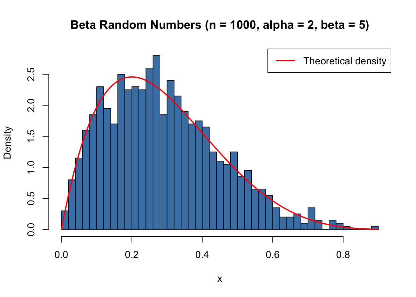
set.seed(123)x <-rbeta(1000, shape1 =2, shape2 =5)hist(x, breaks =35, col ="steelblue", freq =FALSE,xlab ="x", main ="Beta Random Numbers (n = 1000, alpha = 2, beta = 5)")curve(dbeta(x, shape1 =2, shape2 =5), add =TRUE, col ="red", lwd =2)legend("topright", legend ="Theoretical density", col ="red", lwd =2)
Figure 30.3: Histogram of simulated Beta random numbers (n = 1000, alpha = 2, beta = 5)
The Uniform distribution on \([0,1]\) is the special case \(\alpha = \beta = 1\) (see Chapter 19):
\[
\text{Beta}(1, 1) = \text{U}(0, 1)
\]
30.23 Property 2: Reflection Symmetry
If \(X \sim \text{Beta}(\alpha, \beta)\) then \(1 - X \sim \text{Beta}(\beta, \alpha)\). This reflects the symmetry of the density: swapping the two shape parameters is equivalent to reflecting the distribution about \(x = 1/2\).
30.24 Property 3: Conjugate Prior for Bernoulli and Binomial
The Beta distribution is the conjugate prior for the success probability \(\theta\) in a Bernoulli or Binomial model. If the prior is \(\theta \sim \text{Beta}(\alpha, \beta)\) and \(k\) successes are observed in \(n\) trials, the posterior is:
\[
\theta \mid k \sim \text{Beta}(\alpha + k,\; \beta + n - k)
\]
This closed-form Bayesian updating rule is the basis of the Bayesian approach to proportion estimation (see Chapter 7 and Chapter 113).
30.25 Related Distributions 1: Uniform Distribution
\(\text{Beta}(1, 1)\) is the Uniform distribution on \([0,1]\) (see Chapter 19).
30.26 Related Distributions 2: Bayesian Inference for Proportions
The Beta distribution is the natural prior and posterior for the success probability in Bernoulli experiments. See Chapter 7 for the theorem-level framework and Chapter 113 for decision-focused Bayesian workflows.
30.27 Related Distributions 3: Arcsine Distribution
\(\text{Beta}(1/2,\, 1/2)\) is the arcsine distribution with density \(f(x) = 1/(\pi\sqrt{x(1-x)})\). This distribution arises in the study of random walks and the fraction of time a Brownian motion spends above zero.
30.28 Related Distributions 4: Relation to the F-Distribution
If \(X \sim \text{Beta}(\alpha, \beta)\), then \(Y = \frac{\beta}{\alpha}\cdot\frac{X}{1-X} \sim \text{F}(2\alpha, 2\beta)\). This relationship connects the Beta and Fisher F distributions and underpins the exact tail-probability calculations for the F variate.
30.29 Related Distributions 5: Dirichlet Distribution
The Beta distribution is the two-dimensional special case of the Dirichlet: \(\text{Dir}(\alpha_1, \alpha_2) = \text{Beta}(\alpha_1, \alpha_2)\). More generally, each marginal of a Dirichlet vector follows a Beta distribution (see Chapter 44).