glm(count ~ x1 + x2 + offset(log(exposure)), family = poisson, data = df)137 Generalized Linear Models
137.1 The GLM Framework
Generalized Linear Models (GLMs) extend ordinary linear regression to handle response variables that follow distributions other than the normal distribution (Nelder and Wedderburn 1972). A GLM consists of three components:
- Random component: The probability distribution of the response variable \(Y\) (e.g., Normal, Poisson, Binomial)
- Systematic component: The linear predictor \(\eta = \beta_0 + \beta_1 X_1 + ... + \beta_k X_k\)
- Link function: A function \(g(\cdot)\) that relates the expected value of \(Y\) to the linear predictor: \(g(\mu) = \eta\)
Ordinary linear regression (Chapter 134) is a special case of the GLM framework with a Gaussian (normal) family and identity link function. Logistic regression (Chapter 136) is another special case with a binomial family and logit link function.
137.1.1 Common GLM Families
| Family | Link Function | Response Type | Example |
|---|---|---|---|
| Gaussian | Identity: \(g(\mu) = \mu\) | Continuous, symmetric | Height, temperature |
| Binomial | Logit: \(g(\mu) = \log\frac{\mu}{1-\mu}\) | Binary (0/1) or proportions | Disease status, pass/fail |
| Poisson | Log: \(g(\mu) = \log(\mu)\) | Counts (0, 1, 2, …) | Number of accidents, species count |
| Quasipoisson | Log: \(g(\mu) = \log(\mu)\) | Overdispersed counts | Counts with extra variability |
| Negative Binomial | Log: \(g(\mu) = \log(\mu)\) | Overdispersed counts | Species abundance |
| Quasibinomial | Logit: \(g(\mu) = \log\frac{\mu}{1-\mu}\) | Overdispersed proportions | Test scores as proportions |
| Gamma | Inverse: \(g(\mu) = 1/\mu\) | Positive continuous, right-skewed | Insurance claims, waiting times |
Notes:
- Negative binomial regression is widely taught alongside GLMs but is not a strict canonical GLM in the narrow sense because an extra dispersion parameter is estimated.
- For Gamma models, the inverse link is canonical, while the log link is often preferred in applied work because coefficient interpretation is more straightforward.
137.1.2 The General GLM Equation
For a GLM with link function \(g\):
\[ g(E[Y | X]) = \beta_0 + \beta_1 X_1 + \beta_2 X_2 + ... + \beta_k X_k \]
The inverse of the link function maps the linear predictor back to the scale of the response:
\[ E[Y | X] = g^{-1}(\beta_0 + \beta_1 X_1 + ... + \beta_k X_k) \]
137.2 Poisson Regression
137.2.1 When to Use
Poisson regression is used when the response variable represents count data – the number of times an event occurs in a fixed period of time, area, or other unit of observation. Examples include:
- Number of customer complaints per month
- Number of species observed in a habitat
- Number of accidents at an intersection per year
- Number of goals scored per match
The key assumption is that the variance of the counts is approximately equal to the mean (equidispersion).
137.2.2 The Model
The Poisson regression model uses a log link function:
\[ \log(\mu) = \beta_0 + \beta_1 X_1 + \beta_2 X_2 + ... + \beta_k X_k \]
where \(\mu = E[Y | X]\) is the expected count. Equivalently:
\[ \mu = e^{\beta_0 + \beta_1 X_1 + ... + \beta_k X_k} \]
137.2.3 Offsets for Exposure
When observations have different exposure times (e.g., person-years, machine-hours), a Poisson model should include an offset:
\[ \log(\mu_i) = \beta_0 + \beta_1 X_{i1} + \cdots + \beta_k X_{ik} + \log(\text{exposure}_i) \]
In R:
This models event rates rather than raw counts, which is essential when exposure differs across units.
137.2.4 Interpretation of Coefficients
Because of the log link, the coefficients have a multiplicative interpretation:
- A one-unit increase in \(X_j\) multiplies the expected count by \(e^{\beta_j}\)
- The quantity \(e^{\beta_j}\) is called the incidence rate ratio (IRR)
- \(e^{\beta_j} > 1\): the predictor increases the expected count
- \(e^{\beta_j} = 1\): no effect (equivalent to \(\beta_j = 0\))
- \(e^{\beta_j} < 1\): the predictor decreases the expected count
137.2.5 Analysis based on p-values – Software
The Poisson GLM is available in the Manual Model Building application under the GLM tab by selecting “family = poisson”:
137.2.6 R Code
# Example: Number of awards by math score and program type
set.seed(42)
n <- 200
math_score <- round(rnorm(n, mean = 52, sd = 10))
program <- sample(c("General", "Academic", "Vocational"), n, replace = TRUE,
                  prob = c(0.4, 0.35, 0.25))

# True relationship
log_mean <- -3 + 0.04 * math_score + ifelse(program == "Academic", 0.5,
                                              ifelse(program == "Vocational", -0.3, 0))
num_awards <- rpois(n, lambda = exp(log_mean))

df <- data.frame(num_awards, math_score, program = factor(program))

cat("Summary of award counts:\n")
print(table(num_awards))

# Fit Poisson regression
pois_model <- glm(num_awards ~ math_score + program, family = poisson, data = df)
summary(pois_model)
Summary of award counts:
num_awards
0 1 2 3
129 50 20 1
Call:
glm(formula = num_awards ~ math_score + program, family = poisson,
data = df)
Coefficients:
Estimate Std. Error z value Pr(>|z|)
(Intercept) -3.20136 0.64460 -4.966 6.82e-07 ***
math_score 0.04916 0.01105 4.450 8.59e-06 ***
programGeneral -0.23964 0.22653 -1.058 0.2901
programVocational -0.58520 0.30504 -1.918 0.0551 .
---
Signif. codes: 0 '***' 0.001 '**' 0.01 '*' 0.05 '.' 0.1 ' ' 1
(Dispersion parameter for poisson family taken to be 1)
Null deviance: 204.47 on 199 degrees of freedom
Residual deviance: 179.57 on 196 degrees of freedom
AIC: 342.84
Number of Fisher Scoring iterations: 5# Incidence rate ratios (IRR)
cat("\nIncidence Rate Ratios (IRR) with 95% CI:\n")
irr <- exp(cbind(IRR = coef(pois_model), confint(pois_model)))
print(irr)
Incidence Rate Ratios (IRR) with 95% CI:
                         IRR      2.5 %    97.5 %
(Intercept)       0.04070667 0.01125596 0.1409211
math_score        1.05039279 1.02795544 1.0734627
programGeneral    0.78690986 0.50427827 1.2300309
programVocational 0.55699706 0.29703951 0.9914422
137.2.7 Checking for Overdispersion
A critical assumption of Poisson regression is that the variance equals the mean. When the variance exceeds the mean, we have overdispersion. The dispersion parameter can be estimated as:
\[ \hat{\phi} = \frac{\text{Residual deviance}}{\text{Residual degrees of freedom}} \]
If \(\hat{\phi} \approx 1\), the Poisson model is appropriate. If \(\hat{\phi} \gg 1\), overdispersion is present and the standard errors from the Poisson model will be too small, leading to inflated significance.
# Check dispersion
dispersion <- pois_model$deviance / pois_model$df.residual
cat("Estimated dispersion parameter:", round(dispersion, 3), "\n")
cat("If this value is much larger than 1, consider quasipoisson or negative binomial.\n")
Estimated dispersion parameter: 0.916
If this value is much larger than 1, consider quasipoisson or negative binomial.137.2.8 Assumptions
- The response variable is a count (non-negative integer)
- Observations are independent
- The mean equals the variance (equidispersion)
- The log of the mean is a linear function of the predictors
- No excess zeros beyond what the Poisson distribution predicts
137.3 Overdispersion and Alternatives
When the variance of the count data exceeds the mean (overdispersion), the standard Poisson model is inappropriate because it underestimates the standard errors. Two common alternatives address this problem.
137.3.1 Quasipoisson Regression
Quasipoisson regression handles overdispersion by introducing a dispersion parameter \(\phi\) that scales the variance:
\[ \text{Var}(Y) = \phi \cdot \mu \]
When \(\phi = 1\), this reduces to Poisson regression. When \(\phi > 1\), the standard errors are inflated by \(\sqrt{\phi}\), correctly accounting for the extra variability.
Key properties:
- Same point estimates for coefficients as Poisson regression
- Larger standard errors (more conservative p-values)
- The dispersion parameter \(\phi\) is estimated from the data
- AIC is not available for quasi-families (use F-tests for model comparison)
137.3.1.1 R Code
# Simulate overdispersed count data
set.seed(42)
n <- 200
x <- rnorm(n, mean = 5, sd = 2)
# Overdispersed counts: add extra variability
lambda <- exp(0.5 + 0.3 * x)
y_overdispersed <- rnbinom(n, mu = lambda, size = 2)  # Negative binomial generates overdispersion

df_od <- data.frame(y = y_overdispersed, x = x)

# Standard Poisson (will underestimate SE)
pois_fit <- glm(y ~ x, family = poisson, data = df_od)

# Quasipoisson (corrects SE)
qpois_fit <- glm(y ~ x, family = quasipoisson, data = df_od)

cat("=== Poisson Model ===\n")
cat("Dispersion:", round(pois_fit$deviance / pois_fit$df.residual, 3), "\n")
cat("SE for x:", round(summary(pois_fit)$coefficients["x", "Std. Error"], 4), "\n\n")

cat("=== Quasipoisson Model ===\n")
cat("Dispersion:", round(summary(qpois_fit)$dispersion, 3), "\n")
cat("SE for x:", round(summary(qpois_fit)$coefficients["x", "Std. Error"], 4), "\n")
=== Poisson Model ===
Dispersion: 4.555
SE for x: 0.013
=== Quasipoisson Model ===
Dispersion: 4.854
SE for x: 0.0287 Notice that the quasipoisson model produces larger standard errors, reflecting the true uncertainty more accurately.
137.3.2 Negative Binomial Regression
Negative binomial regression is an alternative approach to overdispersed count data. Instead of adjusting the standard errors post-hoc (as quasipoisson does), it explicitly models the extra variation through a dispersion parameter \(\theta\):
\[ \text{Var}(Y) = \mu + \frac{\mu^2}{\theta} \]
As \(\theta \to \infty\), the negative binomial converges to the Poisson distribution.
Key properties:
- Estimated coefficients may differ slightly from Poisson
- Models the overdispersion mechanism explicitly
- AIC is available for model comparison
- Requires the
MASSpackage in R
137.3.2.1 R Code
# Negative binomial regression
library(MASS)
nb_fit <- glm.nb(y ~ x, data = df_od)
summary(nb_fit)
Call:
glm.nb(formula = y ~ x, data = df_od, init.theta = 2.205366332,
    link = log)

Coefficients:
            Estimate Std. Error z value Pr(>|z|)
(Intercept)  0.63124    0.16083   3.925 8.68e-05 ***
x            0.27417    0.02914   9.409  < 2e-16 ***
---
Signif. codes:  0 '***' 0.001 '**' 0.01 '*' 0.05 '.' 0.1 ' ' 1

(Dispersion parameter for Negative Binomial(2.2054) family taken to be 1)

    Null deviance: 311.22  on 199  degrees of freedom
Residual deviance: 220.96  on 198  degrees of freedom
AIC: 1194.5

Number of Fisher Scoring iterations: 1

              Theta:  2.205
          Std. Err.:  0.296

 2 x log-likelihood:  -1188.486
# Compare all three models
cat("=== Model Comparison ===\n\n")
cat("Poisson AIC:", round(AIC(pois_fit), 1), "\n")
cat("Negative Binomial AIC:", round(AIC(nb_fit), 1), "\n")
cat("(Lower AIC is better; AIC not available for quasipoisson)\n\n")
cat("Coefficient for x:\n")
cat(" Poisson: ", round(coef(pois_fit)["x"], 4),
" (SE:", round(summary(pois_fit)$coefficients["x", "Std. Error"], 4), ")\n")
cat(" Quasipoisson: ", round(coef(qpois_fit)["x"], 4),
" (SE:", round(summary(qpois_fit)$coefficients["x", "Std. Error"], 4), ")\n")
cat(" Negative Binomial: ", round(coef(nb_fit)["x"], 4),
" (SE:", round(summary(nb_fit)$coefficients["x", "Std. Error"], 4), ")\n")=== Model Comparison ===
Poisson AIC: 1599.3
Negative Binomial AIC: 1194.5
(Lower AIC is better; AIC not available for quasipoisson)
Coefficient for x:
Poisson: 0.2653 (SE: 0.013 )
Quasipoisson: 0.2653 (SE: 0.0287 )
Negative Binomial: 0.2742 (SE: 0.0291 )137.3.3 Quasipoisson vs. Negative Binomial: When to Use Which
| Aspect | Quasipoisson | Negative Binomial |
|---|---|---|
| Variance structure | \(\text{Var} = \phi \mu\) (linear in mean) | \(\text{Var} = \mu + \mu^2/\theta\) (quadratic in mean) |
| AIC available | No | Yes |
| Model comparison | F-tests only | AIC, likelihood ratio tests |
| Point estimates | Same as Poisson | May differ from Poisson |
| When to prefer | Mild overdispersion; want simplicity | Moderate to strong overdispersion; need AIC |
137.4 Quasibinomial Regression
Quasibinomial regression extends logistic regression (Chapter 136) to handle overdispersed binary or proportional data. It uses the same logit link function as standard logistic regression but allows the variance to exceed what the binomial distribution predicts.
137.4.1 When to Use
- The response is a proportion (between 0 and 1) rather than a binary outcome
- Binary data shows more variability than the binomial distribution allows
- Cluster-level proportions where within-cluster correlation creates overdispersion
137.4.2 R Code
# Example: Proportion of seeds germinating under different conditions
set.seed(42)
n_plots <- 30
temperature <- rnorm(n_plots, mean = 20, sd = 5)
moisture <- rnorm(n_plots, mean = 50, sd = 10)
seeds_planted <- rep(100, n_plots)

# True germination probability
logit_p <- -2 + 0.1 * temperature + 0.02 * moisture
p <- 1 / (1 + exp(-logit_p))

# Overdispersed binomial (beta-binomial simulation)
alpha_param <- p * 5
beta_param <- (1 - p) * 5
actual_p <- rbeta(n_plots, alpha_param, beta_param)
seeds_germinated <- rbinom(n_plots, seeds_planted, actual_p)

df_germ <- data.frame(
  germinated = seeds_germinated,
  total = seeds_planted,
  temperature = temperature,
  moisture = moisture
)

# Standard binomial
binom_fit <- glm(cbind(germinated, total - germinated) ~ temperature + moisture,
                 family = binomial, data = df_germ)

# Quasibinomial (accounts for overdispersion)
qbinom_fit <- glm(cbind(germinated, total - germinated) ~ temperature + moisture,
                  family = quasibinomial, data = df_germ)

cat("=== Standard Binomial ===\n")
cat("Dispersion:", round(binom_fit$deviance / binom_fit$df.residual, 3), "\n")
printCoefmat(summary(binom_fit)$coefficients, digits = 3)

cat("\n=== Quasibinomial ===\n")
cat("Dispersion:", round(summary(qbinom_fit)$dispersion, 3), "\n")
printCoefmat(summary(qbinom_fit)$coefficients, digits = 3)
=== Standard Binomial ===
Dispersion: 19.216
Estimate Std. Error z value Pr(>|z|)
(Intercept) -2.88608 0.25632 -11.26 <2e-16 ***
temperature 0.05698 0.00660 8.63 <2e-16 ***
moisture 0.04921 0.00391 12.59 <2e-16 ***
---
Signif. codes: 0 '***' 0.001 '**' 0.01 '*' 0.05 '.' 0.1 ' ' 1
=== Quasibinomial ===
Dispersion: 17.655
Estimate Std. Error t value Pr(>|t|)
(Intercept) -2.8861 1.0770 -2.68 0.0124 *
temperature 0.0570 0.0277 2.05 0.0498 *
moisture 0.0492 0.0164 3.00 0.0058 **
---
Signif. codes: 0 '***' 0.001 '**' 0.01 '*' 0.05 '.' 0.1 ' ' 1The quasibinomial model produces wider confidence intervals and more conservative p-values when overdispersion is present.
137.5 Model Selection
137.5.1 AIC Comparison
For true likelihood-based models (Poisson, negative binomial, binomial, Gaussian), the Akaike Information Criterion (AIC) can be used to compare models:
\[ \text{AIC} = -2 \ell(\hat{\beta}) + 2k \]
where \(\ell\) is the log-likelihood and \(k\) is the number of parameters. Lower AIC indicates a better balance between fit and complexity.
Important: AIC is not available for quasi-families (quasipoisson, quasibinomial) because they do not specify a full likelihood. For these models, use F-tests or compare with their non-quasi counterparts.
137.5.2 Likelihood Ratio Tests
Nested models can be compared using likelihood ratio tests:
# Compare nested models
full_model <- glm(y ~ x1 + x2, family = poisson, data = df)
reduced_model <- glm(y ~ x1, family = poisson, data = df)
anova(reduced_model, full_model, test = "Chisq")
For quasi-families, use test = "F" instead:
# For quasi-families
full_model <- glm(y ~ x1 + x2, family = quasipoisson, data = df)
reduced_model <- glm(y ~ x1, family = quasipoisson, data = df)
anova(reduced_model, full_model, test = "F")
137.5.3 Residual Diagnostics for GLMs
GLM residuals differ from ordinary residuals in linear regression. The two most useful types are:
- Deviance residuals: Analogous to residuals in linear regression; for moderate/large counts they are often roughly symmetric around zero, but perfect normality is not expected
- Pearson residuals: Standardized by the expected variance; useful for detecting overdispersion
Code
par(mfrow = c(2, 2))

# Deviance residuals vs fitted
plot(predict(pois_model, type = "response"), residuals(pois_model, type = "deviance"),
     xlab = "Fitted values", ylab = "Deviance residuals",
     main = "Deviance Residuals vs Fitted")
abline(h = 0, lty = 2, col = "red")

# QQ plot of deviance residuals
qqnorm(residuals(pois_model, type = "deviance"), main = "QQ Plot of Deviance Residuals")
qqline(residuals(pois_model, type = "deviance"), col = "red")

# Scale-location plot
plot(predict(pois_model, type = "response"),
     sqrt(abs(residuals(pois_model, type = "deviance"))),
     xlab = "Fitted values", ylab = "√|Deviance residuals|",
     main = "Scale-Location")

# Residuals vs leverage
plot(hatvalues(pois_model), residuals(pois_model, type = "deviance"),
     xlab = "Leverage", ylab = "Deviance residuals",
     main = "Residuals vs Leverage")
abline(h = 0, lty = 2, col = "red")

par(mfrow = c(1, 1))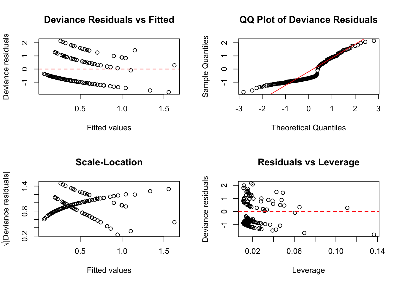
137.6 Assumptions (GLM General)
All GLMs share the following assumptions:
- Correct specification of the link function: The chosen link function correctly relates the mean response to the linear predictor
- Correct distributional family: The response variable follows the specified distribution (or quasi-distribution)
- Independence of observations: Each observation is independent of the others
- No perfect multicollinearity (identification): Predictors cannot be exact linear combinations of each other
- Linearity on the link scale: The relationship between each predictor and the transformed mean is linear
High (imperfect) multicollinearity is a practical estimation concern because it inflates standard errors and can destabilize coefficient estimates.
Additionally, for Poisson models: the mean should equal the variance (unless using quasipoisson or negative binomial).
137.7 Zero-Inflated and Hurdle Extensions
If count data contain many zeros, standard Poisson/negative binomial models can underfit the zero mass. Two common extensions are:
- Zero-inflated models (ZIP/ZINB): combine a point-mass-at-zero component with a count component.
- Hurdle models: model zero vs positive counts first, then positive counts separately.
In R, these can be fit with functions such as pscl::zeroinfl() and pscl::hurdle().
137.8 Pros & Cons
137.8.1 Pros
- Unified framework that encompasses many common regression models
- Handles non-normal response distributions naturally
- Coefficients have interpretable meanings (odds ratios, incidence rate ratios)
- Well-established theory for inference (confidence intervals, hypothesis tests)
- Flexible: can accommodate various response types by choosing the appropriate family
137.8.2 Cons
- Assumes a specific parametric relationship between predictors and response
- Quasi-families do not support AIC-based model comparison
- Overdispersion must be detected and addressed explicitly
- Cannot handle zero-inflated data without extensions (zero-inflated Poisson or hurdle models)
- Requires careful model checking; a poor choice of family or link function leads to invalid inference
137.9 Task
Using the
warpbreaksdataset in R (data(warpbreaks)), fit a Poisson regression model predicting the number of breaks by wool type and tension level. Check for overdispersion. If present, refit using quasipoisson and negative binomial regression and compare the results.Generate overdispersed count data and compare the standard errors from Poisson, quasipoisson, and negative binomial models. Which model gives the most honest standard errors?
Fit a quasibinomial model to proportion data of your choice. Compare the results with a standard binomial model and discuss how overdispersion affects inference.