65  Central Tendency

65.1 Mode

65.1.1 Definition

The Mode of a continuous probability density function (of a variable \(x\)) is the value of \(x\) at which the function reaches its maximum (i.e. the peak of the density function). For discrete distributions, the Mode is the value that is most likely to be sampled.

65.2 Arithmetic Mean

65.2.1 Definition

\[ \bar{x} = \frac{ 1} {n } \sum_{i=1}^{n} x_i \]

65.2.2 Property 1

\[ \frac{ 1} {n } \sum_{i=1}^{n} a = \frac{ 1} {n } n a = a \]

65.2.3 Property 2

\[ \frac{1}{n} \sum_{i=1}^{n} \left( x_i + a \right) = \frac{1}{n} \sum_{i=1}^{n} x_i + \frac{1}{n} n a = \bar{x} + a \]

65.2.4 Property 3

\[ \frac{1}{n} \sum_{i=1}^{n} \left( a x_i \right) = \frac{1}{n} a \sum_{i=1}^{n} x_i = a \bar{x} \]

65.2.5 Property 4

\[ \frac{1}{n} \sum_{i=1}^{n} \left( x_i - \bar{x} \right) = \frac{1}{n} \sum_{i=1}^{n} x_i - \frac{1}{n} \sum_{i=1}^{n} \bar{x} = 0 \]

65.2.6 Standard Deviation of Arithmetic Mean (Population)

\[ \sigma_{\bar{x}} = \frac{\sqrt{\frac{1}{n} \sum_{i=1}^{n} \left( x_i - \bar{x} \right)^2 } }{\sqrt{n} } \]

65.2.7 Standard Deviation of Arithmetic Mean (Sample)

\[ \sigma_{\bar{x}} = \frac{\sqrt{\frac{1}{n-1} \sum_{i=1}^{n} \left( x_i - \bar{x} \right)^2 } }{\sqrt{n} } \]

65.2.8 Pros

The Arithmetic Mean has the following advantages:

• It is easy to compute.
• It is well understood by most readers at the intuitive and mathematical level.
• It can be easily updated when new observations are available (if a new observation becomes available one can easily compute the new mean, without using all previous observations).

65.2.9 Cons

The Arithmetic Mean has the following disadvantages:

• It is sensitive to outliers.
• It assumes that each observation should have an equal weight (this is an implicit assumption which is not always realistic).

65.3 Weighted Mean

65.3.1 Definition

\[ w_x = \sum_{i=1}^{n} \frac{w_i}{ \sum_{j=1}^{n} w_j } x_i \]

65.3.2 Weighted Mean versus Arithmetic Mean

If \(\forall i: w_i = 1\) then \(\sum_{j=1}^{n} w_j = n\) and

\[ w_x = \sum_{i=1}^{n} \frac{w_i}{ \sum_{j=1}^{n} w_j } x_i = \sum_{i=1}^{n} \frac{1}{ n } x_i = \frac{1}{n} \sum_{i=1}^{n} x_i = \bar{x} \]

65.3.3 Pros

The Weighted Mean has the following advantages:

• It is easy to compute.
• It is well understood by educated readers at the intuitive and mathematical level.
• It is possible to attribute low weights to any observation which is uncertain or skews the results (e.g. outliers).

65.3.4 Cons

The Weighted Mean has the following disadvantages:

• It is not always easy to define the weights that should be applied.
• Different weighting schemes yield different results.

65.4 Geometric Mean

65.4.1 Definition

Assuming that \(\forall i: x_i > 0\)

\[ g_x = \sqrt[n]{ \Pi_{i=1}^{n} x_i } \]

\[ \ln g_x = \frac{1}{n} \sum_{i=1}^{n} \ln x_i \]

\[ g_x = e^{\ln g_x} = e^{\frac{1}{n} \sum_{i=1}^{n} \ln x_i} \]

65.4.2 Purpose

The Geometric Mean is mostly used for growth rates, surfaces, and volumes. Whenever we need to multiply observations (growth rates only make sense when being multiplied) then the Geometric Mean should be used rather than the Arithmetic or Weighted Mean.

Within the context of measuring the accuracy of statistical models, the Geometric Mean is sometimes used to express the average of precision and recall (\(G\) score or “Fowlkes-Mallows Index”). More information about the underlying Binomial Classification problem can be found in Chapter 58.

65.4.3 \(G\) score or Fowlkes-Mallows Index

The \(G\) score for a Binomial Classification problem can be computed by applying the definition of the Geometric Mean to the metrics from Chapter 58.

\[ \begin{align*}& G = \sqrt[2]{ \text{Recall} \times \text{Precision} }\end{align*} \]

65.4.4 Example

Suppose we have three investment opportunities:

• Investment 1: +10% in year 1, +10% in year 2, -20% in year 3
• Investment 2: -10% in year 1, -10% in year 2, +20% in year 3
• Investment 3: +30% in year 1, +30% in year 2, -60% in year 3

Which of these opportunities should be preferred? According to the Arithmetic Average, all three investment opportunities have an average growth of 0% which leads us to believe that we are indifferent between them. This conclusion, however, is highly misleading as will be shown below.

Assume that the investment is worth 250 of any currency unit and we first compute the value of each investment at the end of year 1:

• Investment 1 (after 1 year): 250*(1+0.1) = 250*1.1 = 275
• Investment 2 (after 1 year): 250*(1-0.1) = 250*0.9 = 225
• Investment 3 (after 1 year): 250*(1+0.3) = 250*1.3 = 325

At the end of year 2 we have the following net worth for each investment:

• Investment 1 (after 2 years): 275*1.1 = 302.5
• Investment 2 (after 2 years): 225*0.9 = 202.5
• Investment 3 (after 2 years): 325*1.3 = 422.5

Now we compute the net worth at the end of the last year:

• Investment 1 (final value): 302.5*0.8 = 242
• Investment 2 (final value): 202.5*1.2 = 243
• Investment 3 (final value): 422.5*0.4 = 169

The correct answer is that all three investment opportunities are bad (they all make a loss). Investment 2, however, is the best opportunity because it minimizes the loss that is made.

Now we illustrate the fact that the Geometric Mean can be used to obtain the correct answer:

• Investment 1: \(g_x = \sqrt[3]{1.1*1.1*0.8} = 0.9892174886\)
• Investment 2: \(g_x = \sqrt[3]{0.9*0.9*1.2} = 0.9905781747\)
• Investment 3: \(g_x = \sqrt[3]{1.3*1.3*0.4} = 0.8776382955\)

These results are the correct average growth rates for three years. To verify that this is correct one can use the compound interest formula:

• Investment 1 (final value): \(250*0.9892174886^3 = 242\)
• Investment 2 (final value): \(250*0.9905781747^3 = 243\)
• Investment 3 (final value): \(250*0.8776382955^3 = 169\)

65.4.5 Pros

The Geometric Mean has the following advantages:

• It is relatively easy to compute.
• It is reasonably well understood by educated readers.
• It produces the correct result for data observations that need to be multiplied.

65.4.6 Cons

The Geometric Mean has the following disadvantages:

• It is sensitive to outliers.
• It assumes that each observation should have an equal weight (this is an implicit assumption which is not always realistic).

65.5 Harmonic Mean

65.5.1 Definition

\[ h_x = \frac{1}{\frac{1}{n} \sum_{i=1}^{n} \frac{1}{x_i} } = \frac{n}{\sum_{i=1}^{n} \frac{1}{x_i} } \]

\[ h_x^{-1} = \frac{1}{n} \sum_{i=1}^{n} \frac{1}{x_i} \]

65.5.2 Purpose

The Harmonic Mean is typically used for computing the average of output/input ratios. For instance, velocities are expressed as output/input ratios (i.e. distance per time unit) and should be averaged by the Harmonic Mean (this is explained in the Example).

65.5.3 F1 score

Within the context of measuring the accuracy of statistical models, the Harmonic Mean is often used to express the average of precision and recall (\(F_1\) score). More information about the underlying Binomial Classification problem can be found in Chapter 58.

The \(F_1\) score for a Binomial Classification problem can be computed by applying the definition of the Harmonic Mean to the metrics from Chapter 58:

\[ \begin{align*}& F_1 = \frac{1}{\frac{1}{2} \left( \frac{1}{\text{Recall} } + \frac{1}{\text{Precision} } \right) } \\ \\& F_1 = \frac{2}{ \frac{\text{Precision} }{\text{Recall} \times \text{Precision} } + \frac{\text{Recall} }{\text{Recall} \times \text{Precision} } } \\ \\& F_1 = \frac{2}{ \frac{\text{Precision} + \text{Recall} }{\text{Recall} \times \text{Precision} } } \\ \\& F_1 = \frac{2 \times \text{Recall} \times \text{Precision} }{ \text{Precision} + \text{Recall} }\end{align*} \]

65.5.4 Example

Suppose we have three types of transport available to travel from A to B and back. We wish to compute the average speed for each type of transport:

• Transport 1: 50 kilometers per hour from A to B and 100 kilometers per hour from B to A
• Transport 2: 75 kilometers per hour from A to B and back
• Transport 3: 80 kilometers per hour from A to B and 70 kilometers per hour from B to A

The Arithmetic Average is the same for each situation and leads us to believe that the average speed is the same. This, however, is misleading as will be shown below.

The distance between A and B does not matter but for the sake of convenience we will assume that it is 75km. Hence, we can compute the time it takes to travel the whole distance in each case:

• Transport 1:

  • from A to B: 50 km/h = 50/60 km/min = 75/x km/min \(\Rightarrow\) x = 75*6/5 min = 90 minutes
  • form B to A: 100 km/h = 100/60 km/min = 75/x km/min \(\Rightarrow\) x = 75*6/10 min = 45 minutes

• Transport 2: 120 minutes

• Transport 3:

  • from A to B: 75*6/8 = 56.25 minutes
  • from B to A: 75*6/7 \(\simeq\) 64.29 minutes

The travel times for each transport are: 135 min, 120 min, and 120.54 min respectively. Hence the average speeds are: 66.667, 75, and 74.667 km/h. Clearly the three transports have different average speeds and transport 2 is fastest. Also note that transport 3 is much faster than transport 1 (it is almost as fast as transport 2).

Now that we know the correct answer, let us compute the Harmonic Means:

• Transport 1: \(h_x = \frac{1}{\frac{1}{2} \left(\frac{1}{50} + \frac{1}{100}\right)} = 66.6667\)
• Transport 2: \(h_x = \frac{1}{\frac{1}{2} \left(\frac{1}{75} + \frac{1}{75}\right)} = 75\)
• Transport 3: \(h_x = \frac{1}{\frac{1}{2} \left(\frac{1}{80} + \frac{1}{70}\right)} = 74.6667\)

This clearly illustrates the usefulness of the Harmonic Mean. Note that we don’t need the actual distance between A and B!

65.5.5 Pros

The Harmonic Mean has the following advantages:

• It is relatively easy to compute.
• It is (more or less) understood by educated readers.
• It produces the correct result for data observations that are expressed as output/input ratios.

65.5.6 Cons

The Harmonic Mean has the following disadvantages:

• It is sensitive to outliers.
• It assumes that each observation should have an equal weight (this is an implicit assumption which is not always realistic).

65.6 Quadratic Mean

65.6.1 Definition

\[ q_x = \sqrt{\frac{1}{n} \sum_{i=1}^{n} x_i^2 } \]

65.6.2 Purpose

The Quadratic Mean is used to find the average of observations which need to be squared to be meaningful (for instance, when we observe errors we are not necessarily interested in the sign of each error).

65.6.3 Pros

The Quadratic Mean has the following advantages:

• It is relatively easy to compute.
• It is (more or less) understood by educated readers.
• It produces the correct result for data observations that need to be squared to be meaningful.

65.6.4 Cons

The Quadratic Mean has the following disadvantages:

• It is sensitive to outliers.
• It assumes that each observation should have an equal weight (this is an implicit assumption which is not always realistic).

65.7 Root Mean Square

65.7.1 Definition

\[ RMS_x = \sqrt{\frac{1}{n} \sum_{i=1}^{n} \left( x_i - c \right)^2 } \]

65.7.2 Purpose

The Root Mean Square has many applications but within the scope of this book it will be mainly used as a property of a prediction model (which is also a Variability measure).

To understand this, we have to consider that \(c\) does not have to be a predetermined constant. In fact, if we define \(c\) as the prediction of \(x\) then \(x_i - c\) (for \(i=1, 2, …,n\)) can be thought of as the error of the prediction model. In this context, one often refers to the so-called Root Mean Squared Error (RMSE) which is a quality measure of the prediction model (lower values correspond to better predictions). The Mean Squared Error (MSE) is the arithmetic mean of squared prediction errors and the RMSE is its square root. The fact that errors are squared makes sense because we do not want positive and negative errors to cancel each other out when computing an “average of errors”.

So if we want to predict \(x\) based on \(c\) then we could use a simple prediction model \(x_i = c + e_i\) (for \(i=1,2, …,n\)) where \(c\) is chosen or computed in such a way that \(\sqrt{\frac{1}{n}\sum_{i=1}^{n}e_i^2 }\) is as small as possible.

65.7.3 Example

Consider the following data which have been recorded on a weekly basis: \(\left( 5, 4, 6, 3, 8, 10, 9, 7, 2, 3, 1 \right)\). We wish to create three models based on Central Tendency and compare their prediction quality based on the Mean Squared Error.

The three models are specified as follows:

• Weighted Mean v.1: \(x_i = w_i + e_i\) for \(i=1, 2, …, n\) with \(w_i = 0.6 x_{i-1} + 0.4 x_{i-2}\)
• Weighted Mean v.2: \(x_i = w_i + e_i\) for \(i=1, 2, …, n\) with \(w_i = 0.4 x_{i-1} + 0.3 x_{i-2} + 0.2 x_{i-3} + 0.1 x_{i-4}\)
• Arithmetic Mean: \(x_i = \bar{x} + e_i\) for \(i=1, 2, …, n\)

After waiting for three weeks, we obtain the new observations \(x_{n+1} = 2\), \(x_{n+2} = 1\), \(x_{n+3} = 3\). This allows us to compute the predictions and their associated squared errors:

• Weighted Mean v.1: \(x_{n+1} - e_{n+1} = 0.6*1 + 0.4*3 = 1.8\), \(x_{n+2} - e_{n+2} = 0.6*2 + 0.4*1 = 1.6\), \(x_{n+3} - e_{n+3} = 0.6*1 + 0.4*2 = 1.4\) which implies that \(e_{n+1}^2 = (2-1.8)^2 = 0.04\), \(e_{n+2}^2 = (1-1.6)^2 = 0.36\), \(e_{n+3}^2 = (3-1.4)^2 = 2.56\)
• Weighted Mean v.2: \(x_{n+1} - e_{n+1} = … = 2.4\), \(x_{n+2} - e_{n+2} = … = 1.9\), \(x_{n+3} - e_{n+3} = … = 1.5\) which implies that \(e_{n+1}^2 = (2-2.4)^2 = 0.16\), \(e_{n+2}^2 = (1-1.9)^2 = 0.81\), \(e_{n+3}^2 = (3-1.5)^2 = 2.25\)
• Arithmetic Mean: \(x_{n+1} - e_{n+1} = … \simeq 5.2727\), \(x_{n+2} - e_{n+2} = … \simeq 5.2727\), \(x_{n+3} - e_{n+3} = … \simeq 5.2727\) which implies that \(e_{n+1}^2 = (2-5.2727)^2 \simeq 10.71\), \(e_{n+2}^2 = (1-5.2727)^2 \simeq 18.26\), \(e_{n+3}^2 = (3-5.2727)^2 \simeq 5.17\)

The Mean Squared Errors (MSE) can be easily computed for each model:

• MSE of Weighted Mean v.1 \(\simeq 0.98667\)
• MSE of Weighted Mean v.2 \(\simeq 1.07333\)
• MSE of Arithmetic Mean \(\simeq 11.3774\)

The corresponding RMSE values are \(\sqrt{0.98667} \simeq 0.9933\), \(\sqrt{1.07333} \simeq 1.0360\), and \(\sqrt{11.3774} \simeq 3.3730\).

The first model has the best prediction quality, followed closely by the second model. The model based on the Arithmetic Mean does not perform well in this situation.

65.7.4 Pros

The Root Mean Square has the following advantages:

• It is relatively easy to compute.
• It is (more or less) understood by educated readers.
• It allows us to evaluate to quality of prediction models.

65.7.5 Cons

The Root Mean Square has the following disadvantages:

• It is sensitive to outliers.
• It assumes that each observation should have an equal weight (this is an implicit assumption which is not always realistic).

65.8 Quadratic Mean versus Root Mean Square

If \(c = 0\) then

\[ RMS_x = \sqrt{\frac{1}{n} \sum_{i=1}^{n} \left( x_i - 0 \right)^2 } = \sqrt{\frac{1}{n} \sum_{i=1}^{n} x_i^2 } = q_x \]

65.9 Variance versus Root Mean Square

If \(c = \bar{x}\) then

\[ RMS_x = \sqrt{\frac{1}{n} \sum_{i=1}^{n} \left( x_i - \bar{x} \right)^2 } = \sqrt{V(x)} = \sigma_x \]

The Variance is also a measure of Variability.

65.10 General Mean

65.10.1 Definition

\[ M_r(x) = \left( \frac{\sum_{i=1}^{n} w_i x_i^r}{\sum_{i=1}^{n} w_i} \right)^{1/r} \]

65.10.2 Special Cases

If \(r\to +\infty\) then

\[ \lim_{r\to +\infty} M_r(x) = \max \left( x_1, x_2, ..., x_n \right) = x_{max} \]

If \(r = 2\) then

\[ M_2(x) = q_x \]

If \(r = 1\) then

\[ M_1(x) = \bar{x} \]

If \(r\to 0\) then

\[ \lim_{r\to 0} M_r(x) = \Pi_{i=1}^{n} \left( x_i \right)^{\frac{w_i}{\sum_{j=1}^{n} w_j}} \]

If the weights are normalized so that \(\sum_{j=1}^{n} w_j = 1\), then this reduces to \(\Pi_{i=1}^{n} x_i^{w_i}\) (and matches the geometric-mean notation \(g_x\) when that notation assumes normalized weights).

If \(r = -1\) then

\[ M_{-1}(x) = h_x \]

If \(r\to -\infty\) then

\[ \lim_{r\to -\infty} M_r(x) = \min \left( x_1, x_2, ..., x_n \right) = x_{min} \]

65.11 Relationship between Harmonic Mean, Geometric Mean, and Arithmetic Mean

If \(\forall i: x_i > 0\) then

\[ h_x \leq g_x \leq \bar{x} \]

65.12 Median

65.12.1 Definition

If \(n = 2r + 1\) and if the observations are sorted in ascending order then

\[ M_x = x_{r+1} \]

If \(n = 2r\) and if the observations are sorted in ascending order then

\[ M_x = \frac{ \left( x_r + x_{r+1} \right) }{2} \]

65.12.2 Purpose

The Median is often used as an alternative for the Arithmetic Mean, even though they both have entirely different properties. The Median is robust (i.e. not sensitive to outliers) but the distribution of median values can be quite cumbersome (as will be illustrated in the description of the Bootstrap Plot).

65.12.3 Example

Consider the following data which have been recorded on a weekly basis: \(\left( 5, 4, 6, 3, 8, 100, 9, 7, 2, 3, 1 \right)\). We wish to create two models based on Central Tendency and compare their prediction quality based on the Root Mean Squared Error (Section 65.7).

First we compute both measures of Central Tendency:

• Model based on Arithmetic Mean: \(\bar{x} \simeq 13.4545\)
• Model based on Median: \(M_x = 5\)

These results can now be used to compute the squared errors for the next three observations (\(x_{n+1} = 2\), \(x_{n+2} = 1\), \(x_{n+3} = 3\)):

• Model based on Arithmetic Mean: \(e_{n+1}^2 = (2 - 13.4545)^2 \simeq 131.21\), \(e_{n+2}^2 = (1 - 13.4545)^2 \simeq 155.11\), and \(e_{n+3}^2 = (3 - 13.4545)^2 \simeq 109.30\)
• Model based on Median: \(e_{n+1}^2 = (2 - 5)^2 = 9\), \(e_{n+2}^2 = (1 - 5)^2 = 16\), and \(e_{n+3}^2 = (3 - 5)^2 = 4\)

The approximate Root Mean Squared Errors (see Section 65.7) of the models are \(\sqrt{131.87} \simeq 11.48\) and \(\sqrt{9.667} \simeq 3.11\) respectively. The Median clearly outperforms the Arithmetic Mean in terms of prediction quality (it has a much lower RMSE). The reason for this is because the data set contains an outlier.

65.12.4 Pros

The Median has the following advantages:

• It is relatively easy to compute.
• It is well understood by most readers.
• It is robust (i.e. not sensitive to outliers).

65.12.5 Cons

The Median has the following disadvantages:

• The distribution of Medians is not as easy to describe as the distribution of the Arithmetic Mean.
• It requires the entire data set to be sorted.

65.13 Midrange or Midextreme

65.13.1 Definition

If the observations are sorted in ascending order and if \(j = \left\lfloor \frac{n}{4} \right\rfloor\) then

\[ R_x = \frac{x_{min} + x_{max} } {2} = \frac{x_1 + x_n}{2} \]

65.13.2 Purpose

The Midrange represents the mean of the Uniform Density function.

65.13.3 Pros

The Midrange has the following advantages:

• It is easy to compute.
• It is a much better statistic of Central Tendency than the Arithmetic Mean for Uniform Distributions.

65.13.4 Cons

The Midrange has the following disadvantages:

• It is sensitive to outliers.
• It is a worse statistic of Central Tendency than the Arithmetic Mean for Normal Distributions.

65.14 Midhinge

65.14.1 Definition

If \(Q_1 = Quantile(0.25)\) and \(Q_3 = Quantile(0.75)\) represent the first and third quartile (see Chapter 64) then

\[ H_x = \frac{Q_1 + Q_3}{2} \]

65.14.2 Purpose

The Midhinge is basically the 25% trimmed Midrange (i.e. the Midrange that is obtained after trimming the highest and lowest 25% of observations).

65.14.3 Pros

The Midhinge has the following advantages:

• It has a simple definition and a relatively easy interpretation.
• It is not sensitive to outliers (unlike the Midrange).

65.14.4 Cons

The Midhinge has the following disadvantages:

• Its computation is fairly difficult and depends on the definition of the Quartile that is used (see Chapter 64 on Quartiles).
• It is a worse statistic of Central Tendency than the Arithmetic Mean for Normal Distributions.

65.15 Tukey’s Trimean (Tukey 1977)

65.15.1 Definition

If \(Q_1 = Quantile(0.25)\) and \(Q_3 = Quantile(0.75)\) represent the first and third quartile (see Chapter 64) then

\[ Y_x = \frac{Q_1 + 2 M_x + Q_3}{4} \]

Note: \(M_x = Q_2 = Quantile(0.5)\) (= second quartile = median).

65.15.2 Purpose

Tukey’s Trimean is a weighted average of the Median, the first Quartile and the third Quartile. Hence, it combines the information from the Median and the Midhinge.

65.15.3 Pros

Tukey’s Trimean has the following advantages:

• It has a simple definition and a relatively easy interpretation.
• It is not sensitive to outliers.
• It is a very good estimator of Central Tendency when the number of observations is large and the underlying distribution is symmetric.

65.15.4 Cons

Tukey’s Trimean has the following disadvantages:

• Its computation is fairly difficult and depends on the definition of the Quartile that is used (see Chapter 64 on Quartiles).

• Most readers are not familiar with this statistic (hence it is not often used).

65.16 Midmean

65.16.1 Definition

If the observations are sorted in ascending order and if \(j = \left\lfloor \frac{n}{4} \right\rfloor\) then

\[ N_x = T_{j/n}(x) = \frac{1}{n-2j} \sum_{i=j+1}^{n-j} x_i \]

65.16.2 Purpose

The Midmean is the 25% trimmed mean (using \(j = \left\lfloor \frac{n}{4} \right\rfloor\) observations trimmed from each tail), a special case of the Trimmed Mean discussed below.

65.17 The \(\left( j/n \right)^{th}\) Trimmed Mean

65.17.1 Definition

If the observations are sorted in ascending order then

\[ T_{j/n}(x) = \frac{1}{n-2j} \sum_{i=j+1}^{n-j} x_i \]

65.17.2 Horizontal axis

The horizontal axis shows the value of \(j\) (i.e. the number of values that are trimmed on the left and right sides of the distribution).

65.17.3 Vertical axis

The vertical axis displays the value of the mean after trimming has been applied.

65.17.4 Example

The plot on the right shows the Trimmed Means for the time needed by students to submit a short survey (in seconds)

Interactive Shiny app (click to load).

Open in new tab

The plot on the left represents the Winsorized Mean (for the same dataset) which is explained in the next section.

65.18 The \(\left( j/n \right)^{th}\) Winsorized Mean (Dixon and Tukey 1968)

65.18.1 Definition

If the observations are sorted in ascending order then

\[ W_{j/n}(x) = \frac{1}{n} \left( j x_{j+1} + \sum_{i=j+1}^{n-j} x_i + j x_{n-j} \right) \]

65.18.2 Horizontal axis

The horizontal axis shows the value of \(j\) (i.e. the number of values that are winsorized on the left and right sides of the distribution).

65.18.3 Vertical axis

The vertical axis displays the value of the mean after winsorizing has been applied.

65.19 R Module

65.19.1 Public website

The Central Tendency module can be found on the public website:

• https://compute.wessa.net/ct.wasp

65.19.2 RFC

The Central Tendency module is available in RFC under the menu item “Descriptive / Central Tendency”.

If you prefer to compute the measures of Central Tendency on your local machine, the following three scripts can be used in the R console:

x <- rnorm(2000, 3, 1) + 100

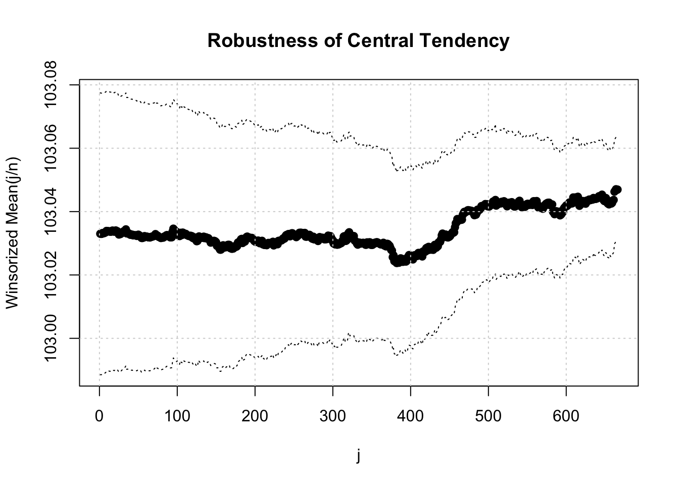
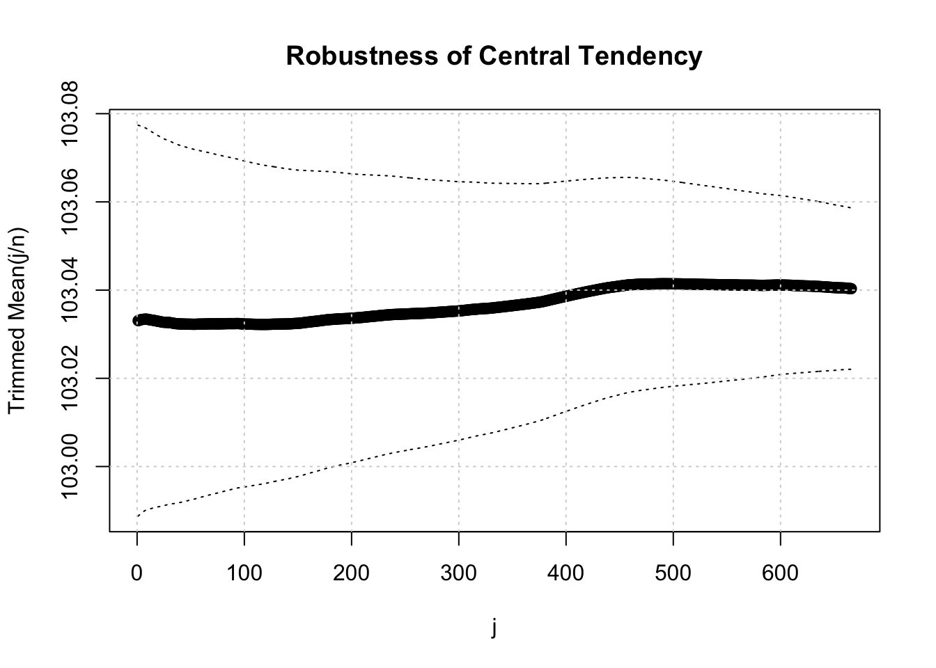
main = 'Robustness of Central Tendency'
geomean <- function(x) {
  return(exp(mean(log(x))))
}
harmean <- function(x) {
  return(1/mean(1/x))
}
quamean <- function(x) {
  return(sqrt(mean(x*x)))
}
winmean <- function(x) {
  x <-sort(x[!is.na(x)])
  n<-length(x)
  denom <- 3
  nodenom <- n/denom
  if (nodenom>40) denom <- n/40
  sqrtn = sqrt(n)
  roundnodenom = floor(nodenom)
  win <- array(NA,dim=c(roundnodenom,2))
  for (j in 1:roundnodenom) {
    win[j,1] <- (j*x[j+1]+sum(x[(j+1):(n-j)])+j*x[n-j])/n
    win[j,2] <- sd(c(rep(x[j+1],j),x[(j+1):(n-j)],rep(x[n-j],j)))/sqrtn
  }
  return(win)
}
trimean <- function(x) {
  x <-sort(x[!is.na(x)])
  n<-length(x)
  denom <- 3
  nodenom <- n/denom
  if (nodenom>40) denom <- n/40
  sqrtn = sqrt(n)
  roundnodenom = floor(nodenom)
  tri <- array(NA,dim=c(roundnodenom,2))
  for (j in 1:roundnodenom) {
    tri[j,1] <- mean(x,trim=j/n)
    tri[j,2] <- sd(x[(j+1):(n-j)]) / sqrt(n-j*2)
  }
  return(tri)
}
midrange <- function(x) {
  return((max(x)+min(x))/2)
}
q1 <- function(data,n,p,i,f) {
  np <- n*p;
  i <<- floor(np)
  f <<- np - i
  qvalue <- (1-f)*data[i] + f*data[i+1]
}
q2 <- function(data,n,p,i,f) {
  np <- (n+1)*p
  i <<- floor(np)
  f <<- np - i
  qvalue <- (1-f)*data[i] + f*data[i+1]
}
q3 <- function(data,n,p,i,f) {
  np <- n*p
  i <<- floor(np)
  f <<- np - i
  if (f==0) {
    qvalue <- data[i]
  } else {
    qvalue <- data[i+1]
  }
}
q4 <- function(data,n,p,i,f) {
  np <- n*p
  i <<- floor(np)
  f <<- np - i
  if (f==0) {
    qvalue <- (data[i]+data[i+1])/2
  } else {
    qvalue <- data[i+1]
  }
}
q5 <- function(data,n,p,i,f) {
  np <- (n-1)*p
  i <<- floor(np)
  f <<- np - i
  if (f==0) {
    qvalue <- data[i+1]
  } else {
    qvalue <- data[i+1] + f*(data[i+2]-data[i+1])
  }
}
q6 <- function(data,n,p,i,f) {
  np <- n*p+0.5
  i <<- floor(np)
  f <<- np - i
  qvalue <- data[i]
}
q7 <- function(data,n,p,i,f) {
  np <- (n+1)*p
  i <<- floor(np)
  f <<- np - i
  if (f==0) {
    qvalue <- data[i]
  } else {
    qvalue <- (1-f)*data[i] + f*data[i+1]
  }
}
q8 <- function(data,n,p,i,f) {
  np <- (n+1)*p
  i <<- floor(np)
  f <<- np - i
  if (f==0) {
    qvalue <- data[i]
  } else {
    if (f == 0.5) {
      qvalue <- (data[i]+data[i+1])/2
    } else {
      if (f < 0.5) {
      qvalue <- data[i]
      } else {
        qvalue <- data[i+1]
      }
    }
  }
}
midmean <- function(x,def) {
  x <-sort(x[!is.na(x)])
  n<-length(x)
  if (def==1) {
    qvalue1 <- q1(x,n,0.25,i,f)
    qvalue3 <- q1(x,n,0.75,i,f)
  }
  if (def==2) {
    qvalue1 <- q2(x,n,0.25,i,f)
    qvalue3 <- q2(x,n,0.75,i,f)
  }
  if (def==3) {
    qvalue1 <- q3(x,n,0.25,i,f)
    qvalue3 <- q3(x,n,0.75,i,f)
  }
  if (def==4) {
    qvalue1 <- q4(x,n,0.25,i,f)
    qvalue3 <- q4(x,n,0.75,i,f)
  }
  if (def==5) {
    qvalue1 <- q5(x,n,0.25,i,f)
    qvalue3 <- q5(x,n,0.75,i,f)
  }
  if (def==6) {
    qvalue1 <- q6(x,n,0.25,i,f)
    qvalue3 <- q6(x,n,0.75,i,f)
  }
  if (def==7) {
    qvalue1 <- q7(x,n,0.25,i,f)
    qvalue3 <- q7(x,n,0.75,i,f)
  }
  if (def==8) {
    qvalue1 <- q8(x,n,0.25,i,f)
    qvalue3 <- q8(x,n,0.75,i,f)
  }
  midm <- 0
  myn <- 0
  roundno4 <- round(n/4)
  round3no4 <- round(3*n/4)
  for (i in 1:n) {
    if ((x[i]>=qvalue1) & (x[i]<=qvalue3)){
      midm = midm + x[i]
      myn = myn + 1
    }
  }
  midm = midm / myn
  return(midm)
}

midm <- array(NA,dim=8)
for (j in 1:8) midm[j] <- midmean(x,j) #Midmean for various types of quantiles
win <- winmean(x)
tri <- trimean(x)
df = data.frame(Statistic = c("Arithmetic Mean",
                              "SD of Arithmetic Mean",
                              "t-value",
                              "Geometric Mean",
                              "Harmonic Mean",
                              "Quadratic Mean",
                              "Median",
                              "Midrange",
                              "Midmean for various quartiles (def 1)",
                              "Midmean for various quartiles (def 2)",
                              "Midmean for various quartiles (def 3)",
                              "Midmean for various quartiles (def 4)",
                              "Midmean for various quartiles (def 5)",
                              "Midmean for various quartiles (def 6)",
                              "Midmean for various quartiles (def 7)",
                              "Midmean for various quartiles (def 8)"),
                Value = c(arm <- mean(x),
                          armse <- sd(x) / sqrt(length(x)),
                          arm / armse,
                          geomean(x),
                          harmean(x),
                          quamean(x),
                          median(x),
                          midrange(x),
                          midm[1],
                          midm[2],
                          midm[3],
                          midm[4],
                          midm[5],
                          midm[6],
                          midm[7],
                          midm[8]))
print(df)

                               Statistic        Value
1                        Arithmetic Mean  103.0329656
2                  SD of Arithmetic Mean    0.0222455
3                                t-value 4631.6325817
4                         Geometric Mean  103.0281642
5                          Harmonic Mean  103.0233618
6                         Quadratic Mean  103.0377660
7                                 Median  103.0284379
8                               Midrange  102.9230742
9  Midmean for various quartiles (def 1)  103.0407695
10 Midmean for various quartiles (def 2)  103.0414260
11 Midmean for various quartiles (def 3)  103.0407695
12 Midmean for various quartiles (def 4)  103.0414260
13 Midmean for various quartiles (def 5)  103.0414260
14 Midmean for various quartiles (def 6)  103.0407695
15 Midmean for various quartiles (def 7)  103.0414260
16 Midmean for various quartiles (def 8)  103.0414269

lb <- win[,1] - 2*win[,2]
ub <- win[,1] + 2*win[,2]
plot(win[,1],type='b',main=main, xlab='j', pch=19, ylab='Winsorized Mean(j/n)', ylim=c(min(lb),max(ub)))
lines(ub,lty=3)
lines(lb,lty=3)
grid()

lb <- tri[,1] - 2*tri[,2]
ub <- tri[,1] + 2*tri[,2]
plot(tri[,1],type='b',main=main, xlab='j', pch=19, ylab='Trimmed Mean(j/n)', ylim=c(min(lb),max(ub)))
lines(ub,lty=3)
lines(lb,lty=3)
grid()

To compute the Central Tendency measures, the R code uses several standard functions (these do not require an external library) such as mean and median. The remainder of Central Tendency measures, however, have been defined in separate functions. As an alternative, if one does not wish to write custom functions, it is possible to find most of these functions in third-party libraries that are published on CRAN (i.e. the official repository of R libraries). Note that the dataset has been defined as a simulation from a Normal Distribution plus a value of 100 to make all values positive (otherwise some functions cannot be computed).

65.20 Purpose of Central Tendency in general

Central Tendency measures are mainly used to summarize univariate variables. As such they are used as a descriptive statistic of the underlying probability distribution. They are extensively used in a wide variety of other statistical methods such as Bootstrap Plots, Mean Plots, Hypothesis Testing, and many types of statistical modeling.

From the Explorative Data Analysis point of view, Central Tendency is used as the parameter of a predictive model. The underlying rationale is that the simplest type of prediction one is able to make about a univariate variable is its measure of Central Tendency. In this sense, the prediction model building process needs to address the following questions:

• Which measure of Central Tendency should be used? For instance, should we use the Arithmetic Mean (for which the predictions can be shown to have a low degree of uncertainty) or the Median (which is not sensitive to outliers)?
• How should the Central Tendency parameter be computed? For instance, what degree of trimming or winsorizing should be applied?
• What is known (or what can be assumed) about the distribution of the prediction error?

65.21 Task

What is the “best” estimate of central tendency about the time needed to submit the survey (use the R module shown in the example of Trimmed and Winsorized Means)?

Dixon, W. J., and J. W. Tukey. 1968. “Approximate Behavior of the Distribution of Winsorized \(t\) (Trimming/Winsorization II).” Technometrics 10: 83–98.

Tukey, John W. 1977. Exploratory Data Analysis. Reading, MA: Addison-Wesley.