69  Notched Boxplot

The box plot was introduced by Tukey (1977) as part of Exploratory Data Analysis. The notched variant was proposed by McGill, Tukey, and Larsen (1978).

69.1 Traditional Boxplot

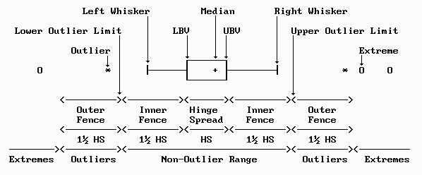
Figure 69.1: Traditional Boxplot -- Example

Figure 69.1 represents an illustration of the traditional boxplot and labels the components of the plot.

69.1.1 Lower Hinge

The Lower Hinge definition is based on Quantiles (see Chapter 64)

\[ LH = Q_1 = Quantile(0.25) \]

69.1.2 Upper Hinge

The Upper Hinge definition is based on Quantiles (see Chapter 64)

\[ UH = Q_3 = Quantile(0.75) \]

69.1.3 Hinge Spread

The Hinge Spread definition is based on Quantiles (see Chapter 64)

\[ HS = UH - LH = Q_3 - Q_1 = Quantile(0.75) - Quantile(0.25) \]

The HS describes the range of that half of the data which sits in the center of the distribution. The highest 25% of the data values lie above this interval. The lowest 25% of the data values lie below the HS. Note: the HS also defines the Interquartile Range (IQR) as defined in Section 66.17.

69.1.4 Lower Whisker

Spans the distance from the Lower Hinge to the smallest observation in the non-outlier range (i.e., the smallest observation at or above \(Q_1 - \frac{3}{2}IQR\)).

69.1.5 Upper Whisker

Spans the distance from the Upper Hinge to the largest observation in the non-outlier range (i.e., the largest observation at or below \(Q_3 + \frac{3}{2}IQR\)).

The fence values are classification thresholds and do not have to coincide with the whisker endpoints.

69.1.6 Lower Inner Fence

Is the interval between the Lower Hinge (\(Q_1\)) and \(Q_1 - \frac{3}{2} IQR\). The Lower Whisker is never larger than the Lower Inner Fence.

69.1.7 Upper Inner Fence

Is the interval between the Upper Hinge (\(Q_3\)) and \(Q_3 + \frac{3}{2} IQR\). The Upper Whisker is never larger than the Upper Inner Fence.

69.1.8 Lower Outer Fence

\[ LOF = \left[ Q_1 - 3 IQR, Q_1 - \frac{3}{2} IQR \right] \]

69.1.9 Upper Outer Fence

\[ UOF = \left[ Q_3 + \frac{3}{2} IQR, Q_3 + 3 IQR \right] \]

69.1.10 Outliers

Data values within the Outer Fences (LOF and UOF) are called outliers.

69.1.11 Extremes

Data values which are below the Lower Outer Fence (LOF) or above the Upper Outer Fence (UOF) are called extremes. Note: sometimes no distinction is made between the extremes and outliers.

Note: base R’s boxplot() documentation commonly refers to all points beyond the whiskers as “outliers”; this chapter follows Tukey’s two-tier terminology and reserves “extremes” for points beyond \(3 IQR\).

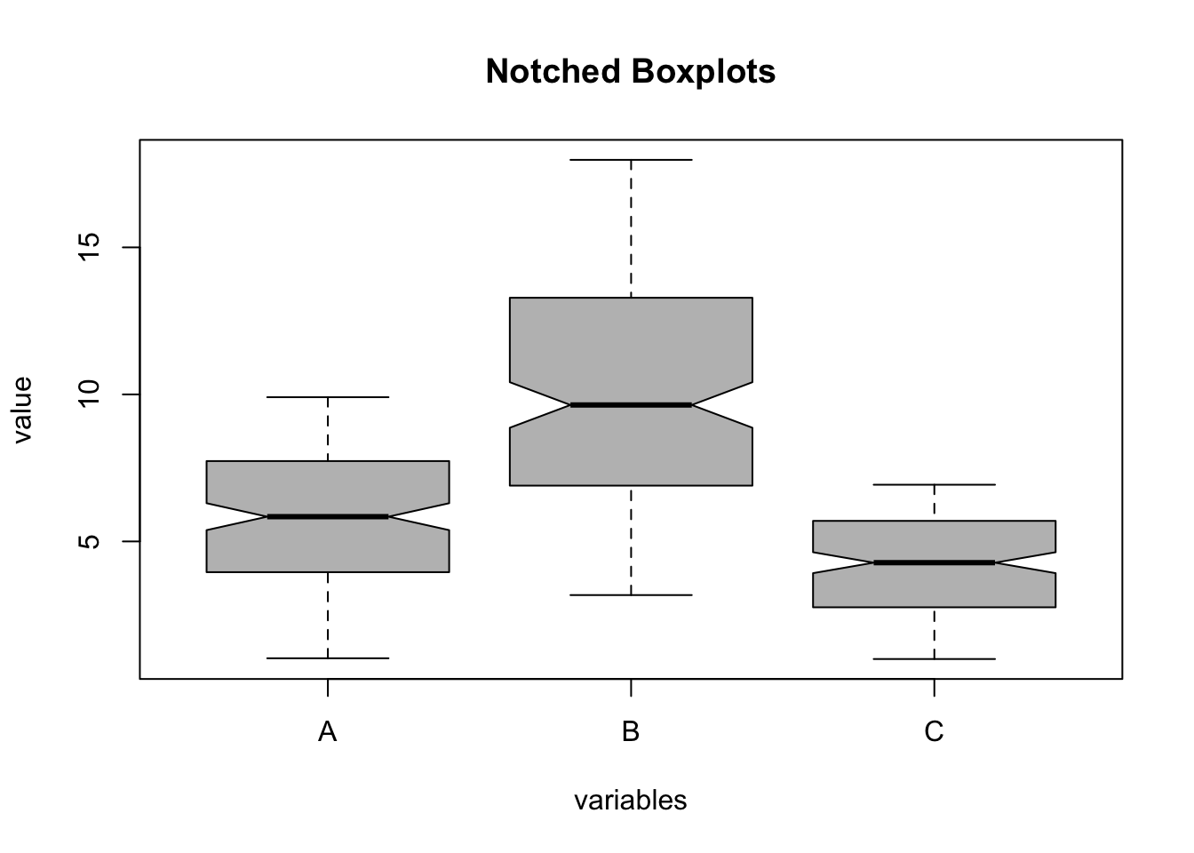
69.1.12 Non-Outlier Range

\[ NOR = \left[ Q_1 - \frac{3}{2} IQR, Q_3 + \frac{3}{2} IQR \right] \]

69.2 Notch of the Boxplot

For the median \(M\), many implementations (including base R) use the following approximate notch interval:

\[ M \pm 1.58 \frac{IQR}{\sqrt{n}} \]

If notches of two boxplots do not overlap, this is often interpreted as evidence that the medians differ.

69.3 R Module

69.3.1 Public website

The Notched Boxplot module can be found on the public website:

• https://compute.wessa.net/rwasp_notchedbox1.wasp

69.3.2 RFC

The Notched Boxplot module is available in RFC under the menu item “Descriptive / Multivariate Descriptive Statistics”.

If you prefer to compute Notched Boxplots on your local machine, the following script can be used in the R console:

A <- runif(170, 1, 10)
B <- runif(170, 3, 18)
C <- runif(170, 1, 7)
x <- cbind(A, B, C)
par1 = 'grey' #colour
par2 = 'no' #omit rows with missing values?
ylab = 'value'
xlab = 'variables'
main = 'Notched Boxplots'
if(par2=='yes') {
  z <- na.omit(x)
} else {
  z <- x
}
r<-boxplot(z ,xlab=xlab,ylab=ylab,main=main,notch=TRUE,col=par1)

boxplot_stats = r$stats
rownames(boxplot_stats) = c('lower whisker', 'lower hinge', 'median', 'upper hinge', 'upper whisker')
colnames(boxplot_stats) = r$names
#Boxplot statistics
boxplot_stats
boxplot_notches = r$conf
rownames(boxplot_notches) = c('lower bound', 'upper bound')
colnames(boxplot_notches) = colnames(boxplot_stats)
#Boxplot notches
boxplot_notches

                     A         B        C
lower whisker 1.026735  3.175745 1.001061
lower hinge   3.954584  6.897660 2.760041
median        5.841958  9.640502 4.277195
upper hinge   7.733022 13.286644 5.699032
upper whisker 9.904877 17.976335 6.928391
                   A         B        C
lower bound 5.384085  8.866282 3.921046
upper bound 6.299830 10.414722 4.633343

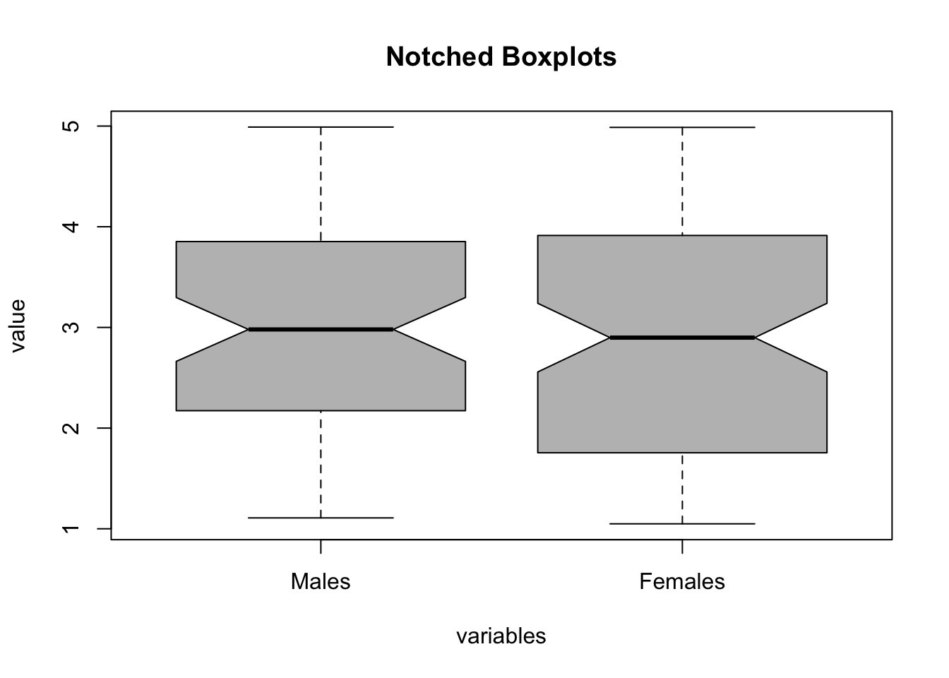
To compute the Notched Boxplots, the R code uses the boxplot function (there is no need for an external library). The second parameter (par2) determines whether the rows with missing values should be eliminated prior to execution through the na.omit function. The boxplot function is one of very few functions in R that works just fine with missing values. To illustrate this we consider the case of scores for female and male students.

Males <- runif(170, 1, 5)
Females <- runif(170, 1, 5)
x <- cbind(Males, Females)
x[1:100,'Males'] = NA
x[101:170,'Females'] = NA
head(x) # show the top section of the data
tail(x) # show the bottom section of the data
par1 = 'grey' #colour
par2 = 'no' #omit rows with missing values?
ylab = 'value'
xlab = 'variables'
main = 'Notched Boxplots'
if(par2=='yes') {
  z <- na.omit(x)
} else {
  z <- x
}
(r<-boxplot(z ,xlab=xlab,ylab=ylab,main=main,notch=TRUE,col=par1))

     Males  Females
[1,]    NA 3.592881
[2,]    NA 4.257305
[3,]    NA 1.324297
[4,]    NA 3.245426
[5,]    NA 1.324153
[6,]    NA 3.966259
          Males Females
[165,] 2.980116      NA
[166,] 3.785962      NA
[167,] 4.304645      NA
[168,] 3.917901      NA
[169,] 3.757140      NA
[170,] 4.559652      NA
$stats
         [,1]     [,2]
[1,] 1.108131 1.049278
[2,] 2.173018 1.755013
[3,] 2.979856 2.898677
[4,] 3.852875 3.913490
[5,] 4.990098 4.987001

$n
[1]  70 100

$conf
         [,1]     [,2]
[1,] 2.662622 2.557637
[2,] 3.297091 3.239716

$out
numeric(0)

$group
numeric(0)

$names
[1] "Males"   "Females"

In the example shown above it is not possible to set par2 = 'yes' because that would delete the entire dataset. There is no need to use na.omit in this case because the boxplot function eliminates the missing values for each column separately which effectively allows us to compare unpaired datasets even if they don’t have the same number of observations (in our example there are more female students).

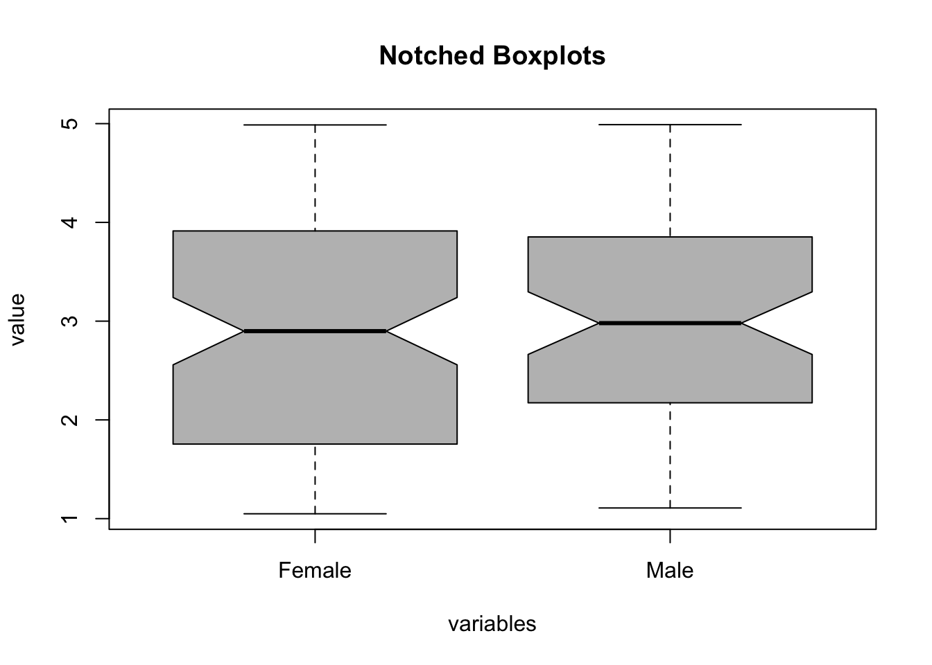
Another important fact to emphasise at this stage is the fact that the data is presented in a so-called “wide” format while it could also have been arranged in a “long” format. This is an example of how we can re-arrange the previous data into long format:

xdf <- data.frame(value = c(x[,"Males"], x[,"Females"]), gender = c(rep("Male", 170), rep("Female", 170)))
boxplot(value ~ gender, data = xdf, xlab = xlab, ylab = ylab, main = main, notch = TRUE, col = par1)

Long format refers to the situation where data has been arranged in “long” columns (observations from females and males are listed in the same column). To ensure that we can still distinguish between both groups, we include a column that represents the categorical variable of the group. The boxplot function allows us to use wide and long format data. In the latter case, however, we must use a so-called “formula” to specify which column contains the actual data and how it depends on the categorical variable: value ~ gender means that we analyse how the value column depends on gender.

69.4 Purpose

Notched Boxplots are very powerful when used correctly. They provide summary statistics about distributional properties of the variables under investigation, including the presence of outliers. Furthermore they can be used to compare and test differences between medians.

69.5 Pros & Cons

69.5.1 Pros

Notched Boxplots have the following advantages:

• They provide a lot of information and are relatively easy to interpret.
• They can be used to detect outliers and excess kurtosis.
• The notches of two or more boxplots can be used to determine whether there is a meaningful difference between two (or more) medians.
• They often provide reliable information about whether the data are skewed or not.

69.5.2 Cons

Notched Boxplots have the following disadvantages:

• They are not well-suited for multi-modal distributions.
• In extreme cases the notches can be larger than the Interquartile Range (this produces funny looking boxplots with “arms” and/or “legs”).

69.6 Example of modern (notched) Boxplots

We have collected survey data based on a 7-point Likert scale and are interested in exploring the first four questions of the survey (labeled Q1_1, Q1_2, Q1_3, and Q1_4). In the analysis shown below we can see:

• the most important descriptive statistics for each Boxplot (Lower Whisker, Lower Hinge, Median, Upper Hinge, and Upper Whisker)
• the Notched Boxplots which are placed side by side and allow us to compare the distributions of answers for each question

Interactive Shiny app (click to load).

Open in new tab

The Notches of the Boxplots can be interpreted as so-called confidence intervals of the median: if two boxes’ notches do not overlap this is ‘strong evidence’ that their medians are different (Chambers et al. (1983), p. 62).

69.7 Task

Based on the R module shown above, compute the boxplots for IM.Know by age.

Chambers, J. M., W. S. Cleveland, B. Kleiner, and P. A. Tukey. 1983. Graphical Methods for Data Analysis. Wadsworth & Brooks/Cole.

McGill, Robert, John W. Tukey, and Wayne A. Larsen. 1978. “Variations of Box Plots.” The American Statistician 32 (1): 12–16. https://doi.org/10.1080/00031305.1978.10479236.

Tukey, John W. 1977. Exploratory Data Analysis. Reading, MA: Addison-Wesley.