89  Blocked Bootstrap Plot (Central Tendency)

The Blocked Bootstrap Plot for Central Tendency uses a special type of bootstrapping (Künsch 1989) which is suited for serially correlated time series. It uses a sliding block of observations to perform the sampling process because this preserves the serial correlation in the simulated time series. In every other aspect, the Blocked Bootstrap Plot is the same as the ordinary Bootstrap Plot which is described in Chapter 83.

89.1 Definition

The Blocked Bootstrap Plot for any given time series \(Y_t\) with \(T\) observations and pre-specified parameter \(k \in \mathbb{N}_0\), is computed according to the following steps:

• generate \(k\) samples \(Z_{jt}\) (for \(j=1,2,…,k\)) of size \(T\) (for \(t = 1, 2, …, T\))
• compute the following measures of Central Tendency: Arithmetic Mean, Median, Midrange, Harmonic Mean, and the Geometric Mean
• compute a series of pre-specified Quantiles such as \(Quantile(q)_j\) for \(q\) = 0.005, 0.025, 0.25, 0.50, 0.75, 0.975, 0.995 and \(j = 1, 2, …,k\)
• plot the simulated statistics
• plot the Gaussian Kernel Density Plots for each simulated statistic
• plot a summary based on Notched Boxplots for each simulated statistic

89.1.1 Horizontal axis for Simulated Statistics

The horizontal axis represents the value of the simulated statistic.

89.1.2 Vertical axis for Simulated Statistics

The vertical axis corresponds to the value of the Central Tendency measure that is drawn from the sample.

89.1.3 Horizontal axis for Kernel Density of Simulated Statistics

The horizontal axis represents the value of the simulated statistic.

89.1.4 Vertical axis for Kernel Density of Simulated Statistics

The vertical axis corresponds to the estimated density value.

89.1.5 Horizontal axis for Notched Boxplots of Simulated Statistics

The horizontal axis represents the measures of Central Tendency (listed in arbitrary order).

89.1.6 Vertical axis for Notched Boxplots of Simulated Statistics

The vertical axis corresponds to the values of the Central Tendency measures.

89.2 Choosing the Block Size

The block size controls how much serial dependence is preserved in each bootstrap sample:

• small blocks preserve only short-run dependence and may underestimate uncertainty
• large blocks preserve more dependence but reduce the effective number of resampled blocks

For monthly data, a block size of 12 is often used as a practical starting point because it preserves one full seasonal cycle. In applied work, compare results for a few nearby block sizes (for example 6, 12, and 18) to check robustness.

89.3 R Module

89.3.1 Public website

The Blocked Bootstrap Plot is available on the public website:

• https://compute.wessa.net/rwasp_bootstrapplot.wasp

89.3.2 RFC

When using the default profile, the Blocked Bootstrap Plot can be found under the “Time Series / Blocked Bootstrap Plot” menu item.

To compute the Blocked Bootstrap Plot on your local machine, the following script can be used in the R console:

library(boot)
library(psych)

x <- cumsum(rnorm(150)) + 100
x = as.ts(x, frequency = 12)
par1 <- 200 # number of simulations
par2 <- 5 # significant digits
par3 <- 12 # blocksize
par4 <- "P0.5 P2.5 Q1 Q3 P97.5 P99.5" # quantiles

boot.stat <- function(s) {
  s.mean <- mean(s)
  s.median <- median(s)
  s.midrange <- (max(s) + min(s)) / 2
  s.hmean <- harmonic.mean(s)
  s.gmean <- geometric.mean(s)
  c(s.mean, s.median, s.midrange, s.hmean, s.gmean)
}

r <- tsboot(x, boot.stat, R = par1, l = par3, sim = "fixed")

z <- data.frame(cbind(r$t[,1],r$t[,2],r$t[,3],r$t[,4],r$t[,5]))
colnames(z) <- list("mean","median","midrange","harmonic","geometric")

if (par4 == "P1 P5 Q1 Q3 P95 P99") {
  myq.1 <- 0.01
  myq.2 <- 0.05
  myq.3 <- 0.95
  myq.4 <- 0.99
}
if (par4 == "P0.5 P2.5 Q1 Q3 P97.5 P99.5") {
  myq.1 <- 0.005
  myq.2 <- 0.025
  myq.3 <- 0.975
  myq.4 <- 0.995
}

df = data.frame(statistic = c("mean",
                              "median",
                              "midrange",
                              "harmonic",
                              "geometric"),
                P1 = c(signif(quantile(r$t[,1],myq.1)[[1]], par2),
                       signif(quantile(r$t[,2],myq.1)[[1]], par2),
                       signif(quantile(r$t[,3],myq.1)[[1]], par2),
                       signif(quantile(r$t[,4],myq.1)[[1]], par2),
                       signif(quantile(r$t[,5],myq.1)[[1]], par2)
                       ),
                P5 = c(signif(quantile(r$t[,1],myq.2)[[1]], par2),
                       signif(quantile(r$t[,2],myq.2)[[1]], par2),
                       signif(quantile(r$t[,3],myq.2)[[1]], par2),
                       signif(quantile(r$t[,4],myq.2)[[1]], par2),
                       signif(quantile(r$t[,5],myq.2)[[1]], par2)
                       ),
                Q1 = c(signif(quantile(r$t[,1],0.25)[[1]], par2),
                       signif(quantile(r$t[,2],0.25)[[1]], par2),
                       signif(quantile(r$t[,3],0.25)[[1]], par2),
                       signif(quantile(r$t[,4],0.25)[[1]], par2),
                       signif(quantile(r$t[,5],0.25)[[1]], par2)
                       ),
                Estimate = c(signif(r$t0[1], par2),
                             signif(r$t0[2], par2),
                             signif(r$t0[3], par2),
                             signif(r$t0[4], par2),
                             signif(r$t0[5], par2)
                             ),
                Q3 = c(signif(quantile(r$t[,1],0.75)[[1]], par2),
                       signif(quantile(r$t[,2],0.75)[[1]], par2),
                       signif(quantile(r$t[,3],0.75)[[1]], par2),
                       signif(quantile(r$t[,4],0.75)[[1]], par2),
                       signif(quantile(r$t[,5],0.75)[[1]], par2)
                       ),
                P95 = c(signif(quantile(r$t[,1],myq.3)[[1]], par2),
                        signif(quantile(r$t[,2],myq.3)[[1]], par2),
                        signif(quantile(r$t[,3],myq.3)[[1]], par2),
                        signif(quantile(r$t[,4],myq.3)[[1]], par2),
                        signif(quantile(r$t[,5],myq.3)[[1]], par2)
                        ),
                P99 = c(signif(quantile(r$t[,1],myq.4)[[1]], par2),
                        signif(quantile(r$t[,2],myq.4)[[1]], par2),
                        signif(quantile(r$t[,3],myq.4)[[1]], par2),
                        signif(quantile(r$t[,4],myq.4)[[1]], par2),
                        signif(quantile(r$t[,5],myq.4)[[1]], par2)
                        ),
                SD = c(signif(sd(r$t[,1]), par2),
                       signif(sd(r$t[,2]), par2),
                       signif(sd(r$t[,3]), par2),
                       signif(sd(r$t[,4]), par2),
                       signif(sd(r$t[,5]), par2)
                       ),
                IQR = c(signif(quantile(r$t[,1],0.75)[[1]] - quantile(r$t[,1],0.25)[[1]], par2),
                        signif(quantile(r$t[,2],0.75)[[1]] - quantile(r$t[,2],0.25)[[1]], par2),
                        signif(quantile(r$t[,3],0.75)[[1]] - quantile(r$t[,3],0.25)[[1]], par2),
                        signif(quantile(r$t[,4],0.75)[[1]] - quantile(r$t[,4],0.25)[[1]], par2),
                        signif(quantile(r$t[,5],0.75)[[1]] - quantile(r$t[,5],0.25)[[1]], par2)
                        )
                ) 
if (par4 == "P0.5 P2.5 Q1 Q3 P97.5 P99.5") {
  colnames(df)[2:3] = c("P0.5", "P2.5")
  colnames(df)[7:8] = c("P97.5", "P99.5")
}

print(df)

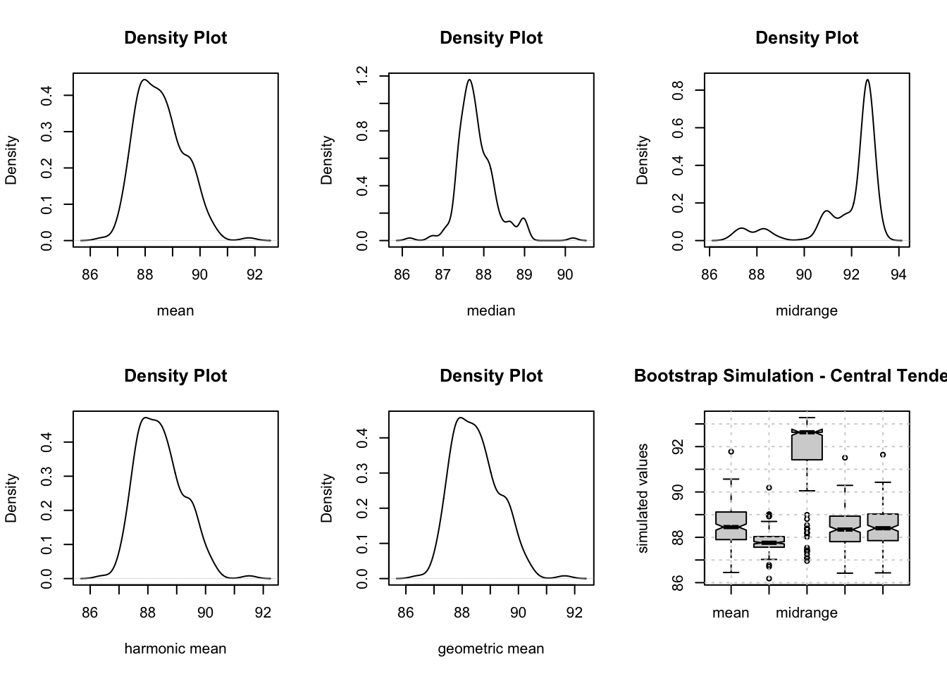
op <- par(mfrow=c(2,3))
plot(density(r$t[,1]),main="Density Plot",xlab="mean")
plot(density(r$t[,2]),main="Density Plot",xlab="median")
plot(density(r$t[,3]),main="Density Plot",xlab="midrange")
plot(density(r$t[,4]),main="Density Plot",xlab="harmonic mean")
plot(density(r$t[,5]),main="Density Plot",xlab="geometric mean")
colnames(z) = c("mean", "median", "midrange", "harmonic", "geometric")
boxplot(z,notch=TRUE,ylab="simulated values",main="Bootstrap Simulation - Central Tendency")

Warning in (function (z, notch = FALSE, width = NULL, varwidth = FALSE, : some
notches went outside hinges ('box'): maybe set notch=FALSE

grid()

par(op)

  statistic   P0.5   P2.5     Q1 Estimate     Q3  P97.5  P99.5      SD     IQR
1      mean 87.095 87.200 87.899   88.495 89.110 90.265 90.572 0.84752 1.21070
2    median 86.704 87.099 87.563   87.712 88.027 88.969 89.020 0.47503 0.46392
3  midrange 87.082 87.382 91.420   92.632 92.632 92.994 92.996 1.57380 1.21240
4  harmonic 87.069 87.180 87.814   88.370 88.933 90.052 90.297 0.79412 1.11940
5 geometric 87.082 87.190 87.857   88.431 89.024 90.157 90.433 0.82017 1.16650

To compute the Blocked Bootstrap Plot, the R code uses the libraries psych and boot. The boot.stat function was created to define all the measures of Central Tendency that are included in the analysis.

89.4 Purpose

The Blocked Bootstrap Plot is used when it is important to compute and compare important Central Tendency measures with empirical confidence intervals. For instance, if we need to assess the quality of a prediction model based on the errors that are produced, by investigating whether or not the Central Tendency of prediction errors is within the range of acceptable levels. In principle, the majority of bootstrap samples (of prediction errors) should yield Central Tendency measures that are around zero. If, for instance, it turns out that more than (say) 95% of samples are on average not equal to zero then we know that the prediction model yields biased forecasts.

89.5 Pros & Cons

89.5.1 Pros

The Blocked Bootstrap Plot has the following advantages:

• It allows one to obtain confidence intervals for Central Tendency measures without the need to know the underlying distribution.
• It provides a lot of useful information about the empirical distribution of the Central Tendency measures.

89.5.2 Cons

The Blocked Bootstrap Plot has the following disadvantages:

• Most readers are not familiar with this type of analysis.
• It cannot be computed with many statistical software packages.

89.6 Example

Consider the prediction errors of a time series forecasting model. We do not want to claim that the average error is exactly equal to zero. Instead, we want to assess whether the bootstrap evidence is consistent with an average prediction error of zero at the chosen 95% confidence level. The practical question is whether the simulated bootstrap samples have Arithmetic Means (and perhaps other measures of Central Tendency) that are plausibly centered around zero, or whether they point to a systematic positive or negative prediction bias.

To examine this question we compute the boundaries of the 95% confidence interval, namely \([Quantile(0.025), Quantile(0.975)]\), and check whether zero remains a plausible value for the average prediction error. If the interval contains zero (that is, the lower bound is negative and the upper bound is positive), then the bootstrap evidence does not support a claim of systematic prediction bias at this confidence level.

Interactive Shiny app (click to load).

Open in new tab

The analysis shows that the Arithmetic Mean is close to zero and that the interval which contains the middle 95% of average prediction errors is approximately equal to [-0.03863, 0.056261]. Since the interval contains zero, the bootstrap results do not provide evidence of a systematic positive or negative average prediction error at the chosen confidence level. Hence, there is no evidence of prediction bias in this example, but this should not be phrased as proof that the true average error is exactly zero.

The Gaussian Kernel Density Plot for the Arithmetic Means of simulated time series shows that most simulated means lie around zero. Which of the five measures of Central Tendency describes the residuals best?

Künsch, Hans R. 1989. “The Jackknife and the Bootstrap for General Stationary Observations.” The Annals of Statistics 17 (3): 1217–41. https://doi.org/10.1214/aos/1176347265.