The Pareto distribution captures the heavy-tail power-law phenomenon seen in income, city sizes, and internet traffic. Its tail decays as \(x^{-\alpha}\) — far slower than the exponential — giving rare extremely large values much more probability than any Normal-family distribution.
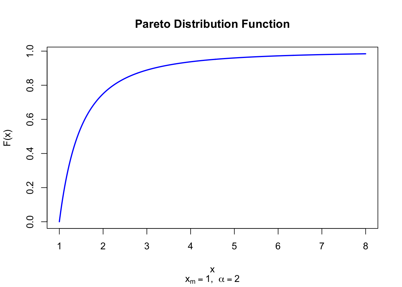
Formally, the random variate \(X\) defined for the range \(X \in [x_m, \infty)\), is said to have a Pareto Distribution (i.e. \(X \sim \text{Pareto}(x_m, \alpha)\)) with minimum value \(x_m > 0\) and shape parameter \(\alpha > 0\). The Pareto distribution does not have a built-in function in base R; custom density and distribution functions are used.
32.1 Probability Density Function
\[
f(x) = \frac{\alpha\, x_m^\alpha}{x^{\alpha+1}}, \quad x \geq x_m
\]
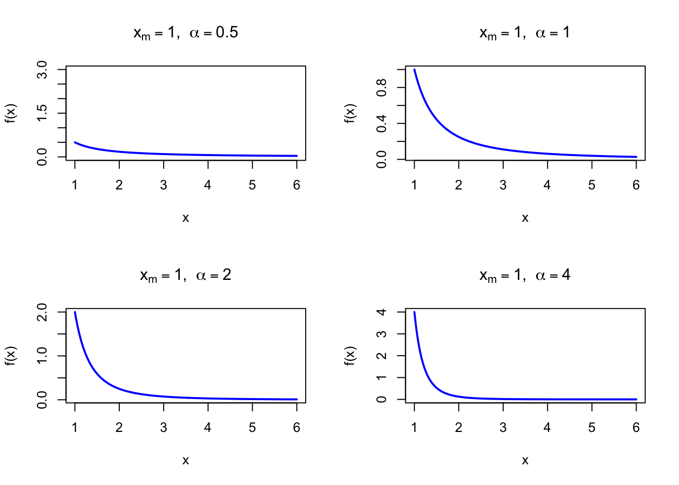
The figure below shows examples of the Pareto Probability Density Function for different shape values with \(x_m = 1\).
Code
dpareto <-function(x, xm, alpha) {ifelse(x >= xm, alpha * xm^alpha / x^(alpha +1), 0)}par(mfrow =c(2, 2))x <-seq(1, 6, length =500)plot(x, dpareto(x, 1, 0.5), type ="l", lwd =2, col ="blue",xlab ="x", ylab ="f(x)", main =expression(paste(x[m] ==1, ", ", alpha ==0.5)),ylim =c(0, 3))plot(x, dpareto(x, 1, 1), type ="l", lwd =2, col ="blue",xlab ="x", ylab ="f(x)", main =expression(paste(x[m] ==1, ", ", alpha ==1)))plot(x, dpareto(x, 1, 2), type ="l", lwd =2, col ="blue",xlab ="x", ylab ="f(x)", main =expression(paste(x[m] ==1, ", ", alpha ==2)))plot(x, dpareto(x, 1, 4), type ="l", lwd =2, col ="blue",xlab ="x", ylab ="f(x)", main =expression(paste(x[m] ==1, ", ", alpha ==4)))par(mfrow =c(1, 1))
Figure 32.1: Pareto Probability Density Function for various shape values (xm = 1)
32.2 Purpose
The Pareto distribution models extreme inequality: the “vital few” observations dominate the total, while the “trivial many” contribute little — the 80/20 rule. Its power-law tail makes it the standard choice for phenomena where the largest values are orders of magnitude larger than typical values. Common applications include:
Income and wealth distributions: a small fraction of individuals hold most wealth
City population sizes: a few mega-cities dwarf the many smaller cities
Internet traffic: a small number of files or users account for most data transfer
Insurance claims: rare catastrophic losses dominate aggregate loss portfolios
Earthquake magnitudes, solar flare intensities, and other natural extreme events
Relation to the discrete setting. The Pareto distribution is the continuous analog of the Zeta (Riemann) distribution, which assigns probability \(\propto k^{-\alpha}\) to positive integers — the theoretical basis of Zipf’s law for word and rank frequencies.
Annual household income (in thousands of USD) above a minimum of \(x_m = 20\)k is modelled as \(X \sim \text{Pareto}(x_m = 20, \alpha = 2.5)\). The mean income is \(\alpha x_m / (\alpha - 1) = 2.5 \times 20 / 1.5 \approx 33.3\)k.
xm <-20; alpha <-2.5ppareto <-function(x, xm, alpha) ifelse(x >= xm, 1- (xm / x)^alpha, 0)# P(X > 50): income exceeds 50kcat("P(income > 50k):", 1-ppareto(50, xm, alpha), "\n")# Mean incomecat("Mean income (k USD):", alpha * xm / (alpha -1), "\n")# Median incomecat("Median income (k USD):", xm *2^(1/alpha), "\n")
P(income > 50k): 0.1011929
Mean income (k USD): 33.33333
Median income (k USD): 26.39016
This means that doubling \(x\) reduces the probability by a factor of \(2^\alpha\), regardless of the starting value — a key signature of scale invariance.
32.23 Property 2: Finite Moments Depend on Shape
Mean exists only for \(\alpha > 1\)
Variance exists only for \(\alpha > 2\)
Skewness is defined only for \(\alpha > 3\)
Kurtosis is defined only for \(\alpha > 4\)
Heavy-tailed phenomena with \(\alpha \leq 2\) are common in practice; for these, sample means and variances are poor estimators.
32.24 Property 3: The 80/20 Rule
Under a Pareto model for wealth distribution, the “80/20 rule” (80% of outcomes come from 20% of causes) corresponds to shape \(\alpha = \log 5 / \log 4 \approx 1.161\).
32.25 Related Distributions 1: Exponential Distribution
If \(X \sim \text{Pareto}(x_m, \alpha)\) then \(\ln(X/x_m) \sim \text{Exp}(\alpha)\) (see Chapter 27). This log-transformation links the two distributions.
32.26 Related Distributions 2: Beta Prime Distribution
The Lomax distribution (shifted Pareto, \(Y = X - x_m\)) is a special case of the Beta Prime distribution with shape1 \(= 1\) (see Chapter 42).
32.27 Related Distributions 3: Fréchet Distribution
The Fréchet distribution governs the maximum of samples from heavy-tailed parent distributions such as the Pareto. Both share power-law tail decay, and the Fréchet shape parameter \(\alpha\) is the reciprocal of the GEV shape \(\xi\) (see Chapter 46).