47  Noncentral t Distribution

The Noncentral t distribution is the key distribution behind statistical power analysis for t-tests. Whenever a researcher asks how many observations do I need? or what is the probability that my study will detect a real effect?, the answer relies on the Noncentral t distribution.

Formally, the random variate \(X\) defined for the range \(-\infty < X < +\infty\), is said to have a Noncentral t Distribution (i.e. \(X \sim \text{t}(n, \delta)\)) with degrees of freedom \(n > 0\) and noncentrality parameter \(\delta \in \mathbb{R}\).

Construction. If \(Z \sim \text{N}(\delta, 1)\) and \(V \sim \chi^2(n)\) are independent, then

\[ T = \frac{Z}{\sqrt{V/n}} \sim \text{t}(n, \delta) \]

When \(\delta = 0\), this reduces to the standard (central) Student t distribution (see Chapter 25). The noncentrality parameter \(\delta\) shifts the distribution away from zero, reflecting the presence of a true effect.

47.1 Probability Density Function

The PDF of the Noncentral t distribution involves a confluent hypergeometric function and does not have a simple closed form. It can be expressed as

\[ f(x) = \frac{n^{n/2} \, e^{-n\delta^2/(2(x^2+n))}}{B\!\left(\frac{1}{2}, \frac{n}{2}\right) (x^2+n)^{(n+1)/2}} \sum_{j=0}^{\infty} \frac{\Gamma\!\left(\frac{n+j+1}{2}\right)}{\Gamma\!\left(\frac{n}{2}\right) \, j!} \left(\frac{x\delta\sqrt{2}}{\sqrt{x^2+n}}\right)^j \]

In practice, R computes the density with dt(x, df, ncp).

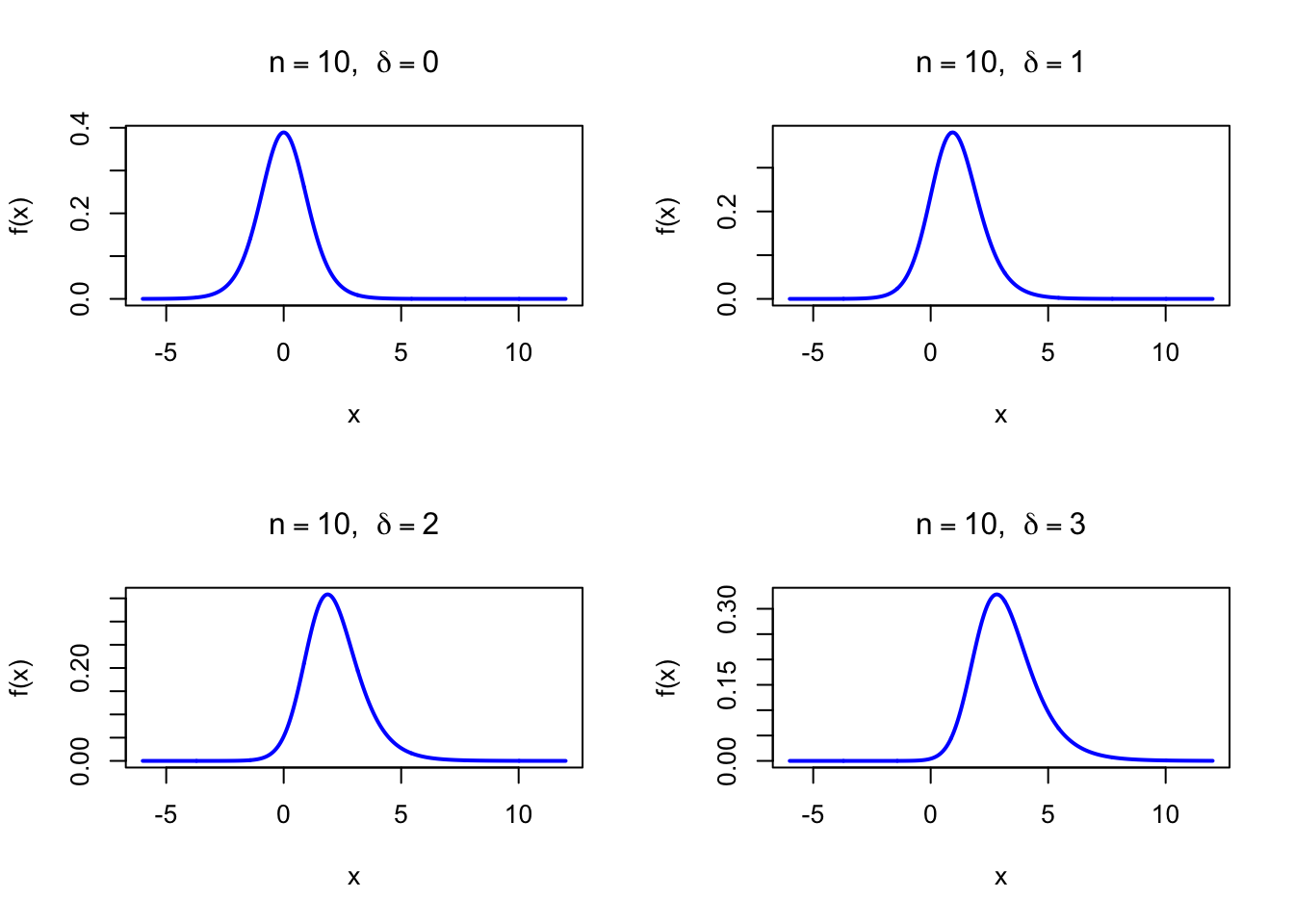
The figure below shows the Noncentral t Probability Density Function for \(n = 10\) and several values of \(\delta\).

par(mfrow = c(2, 2))
x <- seq(-6, 12, length = 1000)

plot(x, dt(x, df = 10, ncp = 0), type = "l", lwd = 2, col = "blue",
     xlab = "x", ylab = "f(x)", main = expression(paste(n == 10, ",  ", delta == 0)))

plot(x, dt(x, df = 10, ncp = 1), type = "l", lwd = 2, col = "blue",
     xlab = "x", ylab = "f(x)", main = expression(paste(n == 10, ",  ", delta == 1)))

plot(x, dt(x, df = 10, ncp = 2), type = "l", lwd = 2, col = "blue",
     xlab = "x", ylab = "f(x)", main = expression(paste(n == 10, ",  ", delta == 2)))

plot(x, dt(x, df = 10, ncp = 3), type = "l", lwd = 2, col = "blue",
     xlab = "x", ylab = "f(x)", main = expression(paste(n == 10, ",  ", delta == 3)))

par(mfrow = c(1, 1))

Figure 47.1: Noncentral t Probability Density Function (df = 10) for various noncentrality values

47.2 Purpose

The Noncentral t distribution is the theoretical backbone of power analysis for t-tests. Its primary applications include:

• Sample size planning: determining how many observations are needed to detect a given effect size with a desired power level
• Power analysis: computing the probability of rejecting the null hypothesis when a true effect of specified size exists
• Clinical trial design: justifying sample sizes in protocols for regulatory submissions
• Grant proposals: providing statistical justification for the planned study size
• Understanding Type II error: quantifying the probability of failing to detect a real effect (\(\beta = 1 - \text{power}\))

Relation to the t-test. Under the null hypothesis (\(H_0: \mu = \mu_0\)), the t statistic follows a central t distribution (with \(\delta = 0\)). Under the alternative hypothesis (\(H_1: \mu = \mu_1 \neq \mu_0\)), the t statistic follows a Noncentral t distribution with a noncentrality parameter that depends on the true effect size and the sample size.

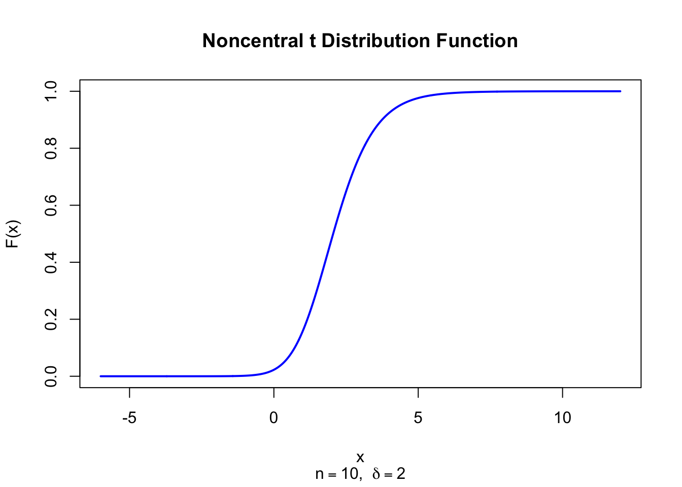
47.3 Distribution Function

There is no elementary closed form for the CDF. It is computed numerically by pt(x, df, ncp) in R.

The figure below shows the Noncentral t Distribution Function for \(n = 10\) and \(\delta = 2\).

x <- seq(-6, 12, length = 1000)
plot(x, pt(x, df = 10, ncp = 2), type = "l", lwd = 2, col = "blue",
     xlab = "x", ylab = "F(x)", main = "Noncentral t Distribution Function",
     sub = expression(paste(n == 10, ",  ", delta == 2)))

Figure 47.2: Noncentral t Distribution Function (df = 10, delta = 2)

47.4 Moment Generating Function

The moment generating function of the Noncentral t distribution does not have a simple closed form. Moments are typically computed from the recursive formulas below.

47.5 Expected Value

\[ \text{E}(X) = \delta \sqrt{\frac{n}{2}} \, \frac{\Gamma\!\left(\frac{n-1}{2}\right)}{\Gamma\!\left(\frac{n}{2}\right)} \quad \text{for } n > 1 \]

For large \(n\), \(\text{E}(X) \approx \delta\).

47.6 Variance

\[ \text{V}(X) = \frac{n(1 + \delta^2)}{n - 2} - \frac{n \delta^2}{2} \left[\frac{\Gamma\!\left(\frac{n-1}{2}\right)}{\Gamma\!\left(\frac{n}{2}\right)}\right]^2 \quad \text{for } n > 2 \]

47.7 Median

There is no closed-form expression for the median. It is computed numerically via qt(0.5, df, ncp) in R:

# Median for t(n = 10, delta = 2)
qt(0.5, df = 10, ncp = 2)

[1] 2.053691

47.8 Mode

The mode of the Noncentral t distribution does not have a simple closed-form expression. It can be found numerically by maximizing the density function. For moderate to large \(n\) and \(\delta > 0\), the mode is approximately equal to \(\delta\).

47.9 Coefficient of Skewness

The Noncentral t distribution is skewed. For \(\delta > 0\) the distribution is right-skewed, and for \(\delta < 0\) it is left-skewed. The skewness depends on both \(n\) and \(\delta\) and does not simplify to a compact formula. It can be computed numerically from the centered moments.

When \(\delta = 0\) (central case), the skewness is zero by symmetry. As \(n \to \infty\), the skewness approaches that of \(\text{N}(\delta, 1)\), which is zero.

47.10 Coefficient of Kurtosis

The kurtosis of the Noncentral t distribution depends on both \(n\) and \(\delta\) and requires \(n > 4\) for existence. It exceeds the Normal kurtosis of 3, indicating heavier tails. As \(n \to \infty\), the kurtosis approaches 3.

47.11 Parameter Estimation

The Noncentral t distribution is not typically fitted to data via parameter estimation in the classical sense. Instead, the noncentrality parameter \(\delta\) is determined from the experimental design:

• One-sample or paired t-test: \(\delta = \sqrt{n} \cdot d\), where \(d = (\mu_1 - \mu_0)/\sigma\) is the standardized effect size and \(n\) is the sample size
• Independent two-sample t-test (equal group sizes): \(\delta = \sqrt{n/2} \cdot d\), where \(d = (\mu_1 - \mu_2)/\sigma\) is Cohen’s \(d\) and \(n\) is the total number of observations per group

Given an observed t statistic, a confidence interval for \(\delta\) can be obtained by inverting the CDF using qt().

47.12 R Module

47.12.1 RFC

The Noncentral t Distribution module is available in RFC under the menu “Distributions / Noncentral t Distribution”.

47.12.2 Direct app link

• https://shiny.wessa.net/nctdist/

47.12.3 R Code

The following code demonstrates Noncentral t probability calculations:

# Probability density function: f(x)
dt(x = 2, df = 10, ncp = 2)

# Distribution function: P(X <= x)
pt(q = 2, df = 10, ncp = 2)

# Quantile function: find x such that P(X <= x) = p
qt(p = 0.975, df = 10, ncp = 2)

# Generate random Noncentral t numbers
set.seed(42)
rt(n = 10, df = 10, ncp = 2)

[1] 0.3556436
[1] 0.4809732
[1] 4.957836
 [1] 2.7175045 0.9830883 3.7032398 2.1186340 2.0594924 1.6528015 3.3237075
 [8] 1.6360023 5.2422904 2.2011690

47.13 Example

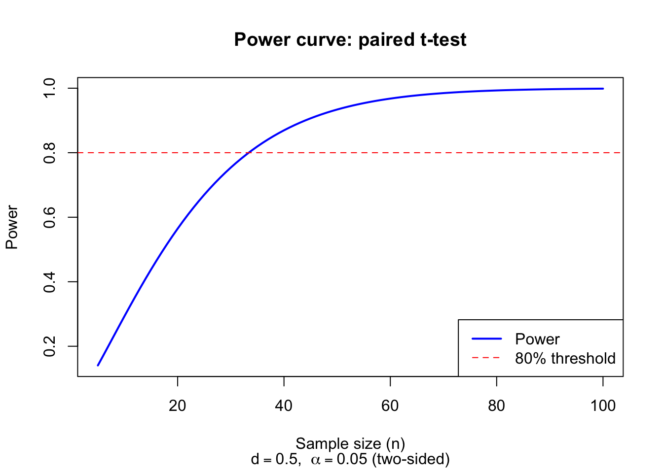
A clinical researcher plans a paired t-test to detect a standardized effect size of \(d = 0.5\) (a medium effect by Cohen’s conventions). Using a two-sided test at \(\alpha = 0.05\), how many subjects are required to achieve 80% power?

The noncentrality parameter for a paired t-test is \(\delta = \sqrt{n} \cdot d\), and the degrees of freedom are \(n - 1\). We compute power for various sample sizes:

d     <- 0.5      # standardized effect size
alpha <- 0.05     # significance level (two-sided)

# Compute power for sample sizes from 10 to 80
n_vals <- seq(10, 80, by = 5)
power  <- numeric(length(n_vals))

for (i in seq_along(n_vals)) {
  n     <- n_vals[i]
  df    <- n - 1
  delta <- sqrt(n) * d
  t_crit <- qt(1 - alpha/2, df = df)
  # Power = P(|T| > t_crit) under the alternative
  power[i] <- 1 - pt(t_crit, df = df, ncp = delta) +
                  pt(-t_crit, df = df, ncp = delta)
}

result <- data.frame(n = n_vals, delta = sqrt(n_vals) * d, power = round(power, 4))
print(result)

# Find minimum sample size for 80% power
n_required <- n_vals[which(power >= 0.80)[1]]
cat("\nMinimum sample size for 80% power:", n_required, "\n")

    n    delta  power
1  10 1.581139 0.2932
2  15 1.936492 0.4379
3  20 2.236068 0.5645
4  25 2.500000 0.6697
5  30 2.738613 0.7540
6  35 2.958040 0.8195
7  40 3.162278 0.8694
8  45 3.354102 0.9066
9  50 3.535534 0.9339
10 55 3.708099 0.9537
11 60 3.872983 0.9678
12 65 4.031129 0.9778
13 70 4.183300 0.9848
14 75 4.330127 0.9896
15 80 4.472136 0.9930

Minimum sample size for 80% power: 35 

d     <- 0.5
alpha <- 0.05
n_vals <- seq(5, 100, by = 1)
power  <- numeric(length(n_vals))
for (i in seq_along(n_vals)) {
  n     <- n_vals[i]
  df    <- n - 1
  delta <- sqrt(n) * d
  t_crit <- qt(1 - alpha/2, df = df)
  power[i] <- 1 - pt(t_crit, df = df, ncp = delta) +
                  pt(-t_crit, df = df, ncp = delta)
}
plot(n_vals, power, type = "l", lwd = 2, col = "blue",
     xlab = "Sample size (n)", ylab = "Power",
     main = "Power curve: paired t-test",
     sub = expression(paste(d == 0.5, ",  ", alpha == 0.05, " (two-sided)")))
abline(h = 0.80, lty = 2, col = "red")
legend("bottomright", legend = c("Power", "80% threshold"),
       col = c("blue", "red"), lty = c(1, 2), lwd = c(2, 1))

Figure 47.3: Power curve for paired t-test (d = 0.5, alpha = 0.05, two-sided)

You can reproduce this analysis interactively using the Noncentral t Distribution app:

Interactive Shiny app (click to load).

Open in new tab

47.14 Random Number Generator

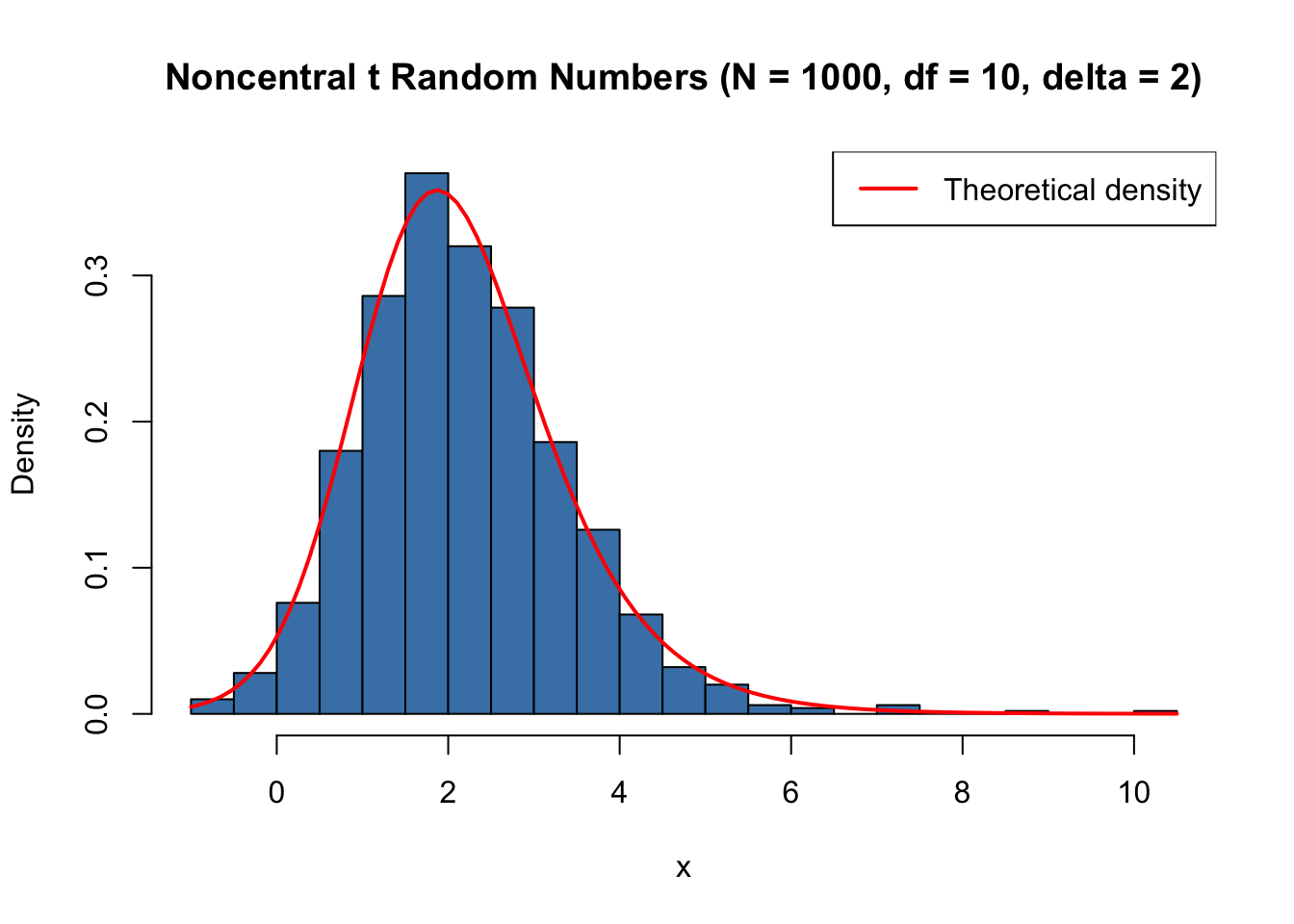
Random variates from the Noncentral t distribution can be generated directly from its construction. If \(Z \sim \text{N}(\delta, 1)\) and \(V \sim \chi^2(n)\) are independent, then \(T = Z / \sqrt{V/n}\) follows \(\text{t}(n, \delta)\).

set.seed(123)
N     <- 1000
n     <- 10
delta <- 2

# Construction method
z <- rnorm(N, mean = delta, sd = 1)
v <- rchisq(N, df = n)
x_construct <- z / sqrt(v / n)

# Built-in function
x_rt <- rt(N, df = n, ncp = delta)

cat("Construction: mean =", round(mean(x_construct), 4),
    "  var =", round(var(x_construct), 4), "\n")
cat("rt():         mean =", round(mean(x_rt), 4),
    "  var =", round(var(x_rt), 4), "\n")

# Theoretical mean
E_theory <- delta * sqrt(n/2) * gamma((n-1)/2) / gamma(n/2)
cat("Theoretical:  mean =", round(E_theory, 4), "\n")

Construction: mean = 2.1936   var = 1.5229 
rt():         mean = 2.1582   var = 1.636 
Theoretical:  mean = 2.1674 

set.seed(123)
x <- rt(1000, df = 10, ncp = 2)
hist(x, breaks = 40, col = "steelblue", freq = FALSE,
     xlab = "x", main = "Noncentral t Random Numbers (N = 1000, df = 10, delta = 2)")
curve(dt(x, df = 10, ncp = 2), add = TRUE, col = "red", lwd = 2)
legend("topright", legend = "Theoretical density", col = "red", lwd = 2)

Figure 47.4: Histogram of simulated Noncentral t random numbers (N = 1000, df = 10, delta = 2)

Interactive Shiny app (click to load).

Open in new tab

47.15 Property 1: Noncentrality and Power

The noncentrality parameter \(\delta\) determines the statistical power of a t-test. Under the alternative hypothesis, the t statistic follows \(\text{t}(n-1, \delta)\) for a one-sample or paired test. Power is the probability that \(|T|\) exceeds the critical value:

\[ \text{Power} = 1 - \text{P}\!\left(-t_{\alpha/2, n-1} \leq T \leq t_{\alpha/2, n-1}\right) \quad \text{where } T \sim \text{t}(n-1, \delta) \]

As \(\delta\) increases (larger effect or larger sample), the Noncentral t density shifts further from zero, and a greater proportion of its area falls beyond the critical values, yielding higher power.

47.16 Property 2: Noncentrality Formulas for t-tests

The noncentrality parameter links the effect size, sample size, and the t distribution:

• One-sample t-test: \(\delta = \sqrt{n} \cdot d\) where \(d = (\mu - \mu_0)/\sigma\)
• Paired t-test: \(\delta = \sqrt{n} \cdot d\) where \(d = \mu_D / \sigma_D\) and \(n\) is the number of pairs
• Independent two-sample t-test (equal groups of size \(n\)): \(\delta = \sqrt{n/2} \cdot d\) where \(d = (\mu_1 - \mu_2)/\sigma_{\text{pooled}}\)

These formulas make it clear that increasing the sample size \(n\) increases \(\delta\) and therefore increases power.

47.17 Property 3: Convergence to Normal

As \(n \to \infty\), the Noncentral t distribution converges to the Normal distribution:

\[ \text{t}(n, \delta) \xrightarrow{d} \text{N}(\delta, 1) \quad \text{as } n \to \infty \]

This follows directly from the construction, since \(\sqrt{V/n} \xrightarrow{p} 1\) as \(n \to \infty\) by the law of large numbers.

47.18 Related Distributions 1: Central t as Special Case

The Student t distribution is the Noncentral t distribution with noncentrality parameter \(\delta = 0\) (see Chapter 25):

\[ \text{t}(n, 0) = \text{t}(n) \]

47.19 Related Distributions 2: Normal as Limiting Case

As \(n \to \infty\), the Noncentral t distribution converges to a Normal distribution with mean \(\delta\) and variance 1:

\[ \text{t}(n, \delta) \xrightarrow{d} \text{N}(\delta, 1) \quad \text{as } n \to \infty \]

47.20 Related Distributions 3: Chi-squared Connection

The construction of the Noncentral t distribution involves a Chi-squared variate in the denominator. Specifically, if \(V \sim \chi^2(n)\) (see Chapter 23), the square root \(\sqrt{V/n}\) provides the scaling.

47.21 Related Distributions 4: Link with the Noncentral F Distribution

The square of a Noncentral t variate with \(n\) degrees of freedom and noncentrality \(\delta\) follows a Noncentral F distribution (see Chapter 48):

\[ T^2 = \text{F}(1, n, \delta^2) \quad \text{where } T \sim \text{t}(n, \delta) \]

This relationship connects power analysis for t-tests to power analysis for F-tests with numerator degrees of freedom equal to 1.

47.22 Related Distributions 5: Noncentral Chi-squared Connection

The noncentrality parameter \(\delta^2\) of the squared Noncentral t variate corresponds to the noncentrality of the Noncentral Chi-squared distribution (see Chapter 24). Specifically, in the numerator of the construction, \(Z^2 \sim \chi^2(1, \delta^2)\) where \(Z \sim \text{N}(\delta, 1)\).