The Quantile-Quantile Plot (QQ Plot) (Wilk and Gnanadesikan 1968) is computed for quantitative data and involves the following computations
a series of Quantiles (as defined in Chapter 64) is computed for the univariate data of interest (called \(x\))
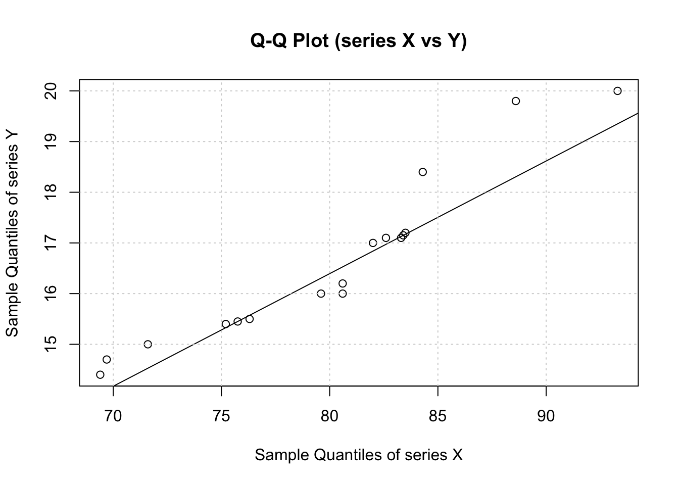
the same Quantiles are also computed for another univariate data series \(y\)
the distributions of both series \(x\) and \(y\) are compared by drawing a scatter plot (see Chapter 70) of their respective Quantiles (the sample sizes do not have to be equal)
a reference line is drawn which identifies the point for which the Quantiles of both data sets are equal
76.2 Vertical axis
The Quantiles of one variable (e.g. \(y\)) are shown on the vertical axis.
76.3 Horizontal axis
The Quantiles of the other variable (e.g. \(x\)) are shown on the horizontal axis.
One often uses Quantiles which correspond to known distributions (instead of empirical data) on one of the axes (e.g. the horizontal axis). This allows the researcher to compare the distribution of a univariate variable against any theoretical distribution. If the theoretical distribution is normal, the plot is called a Normal QQ Plot.
76.4 R Module
76.4.1 Public website
The bivariate QQ Plot can be found on the public website:
qqplot(x,y,main='Q-Q Plot (series X vs Y)',ylab='Sample Quantiles of series Y',xlab='Sample Quantiles of series X')plot.qqline(x,y)grid()
[1] 3 9
[1] 1 3
To compute the bivariate QQ Plot, the R code uses the standard qqplot function from base R. Note that the standard qqline function does not work for bivariate data (it is meant to be used to compare a univariate series against some theoretical distribution). Therefore, the R script defines a new function plot.qqline which allows to plot a line through the scatterplot of the bivariate QQ Plot.
Note that the Normal QQ Plot can be obtained through the base R qqplot function but this is not recommended. Instead, it is better to use the qqPlot function from the car package because it computes the confidence intervals.
76.5 Purpose
The ordinary (bivariate) QQ Plot is simply used to compare the shapes of two empirical distributions. More importantly, however, the QQ Plot can used with only one sample and a theoretical distribution. The Normal QQ Plot is the most prominent plot among all QQ Plots and is used in various types of analysis due to the importance of the Normal Distribution in inferential statistics. Note that the ML Fitting module automatically adapts the QQ Plot to the chosen distribution.
76.6 Pros & Cons
76.6.1 Pros
The QQ Plot has the following advantages:
It can be computed with many software packages.
It is relatively easy to interpret and conveys a lot of information in a simple graph.
Many readers are familiar with QQ Plots -- therefore it is one of the preferred methods to report information about the distribution of a variable of interest.
Unlike the Histogram, QQ Plots do not depend on any parameter (such as a number of bins).
76.6.2 Cons
The QQ Plot has the following disadvantages:
The QQ Plot does not provide unambiguous information about the whether the Quantiles (of both axes) match or not. It is, however, possible to compute the confidence intervals based on bootstrap sampling methods. Note: the car package in R provides these intervals via the qqPlot function (see the R Module section above).
76.7 Example
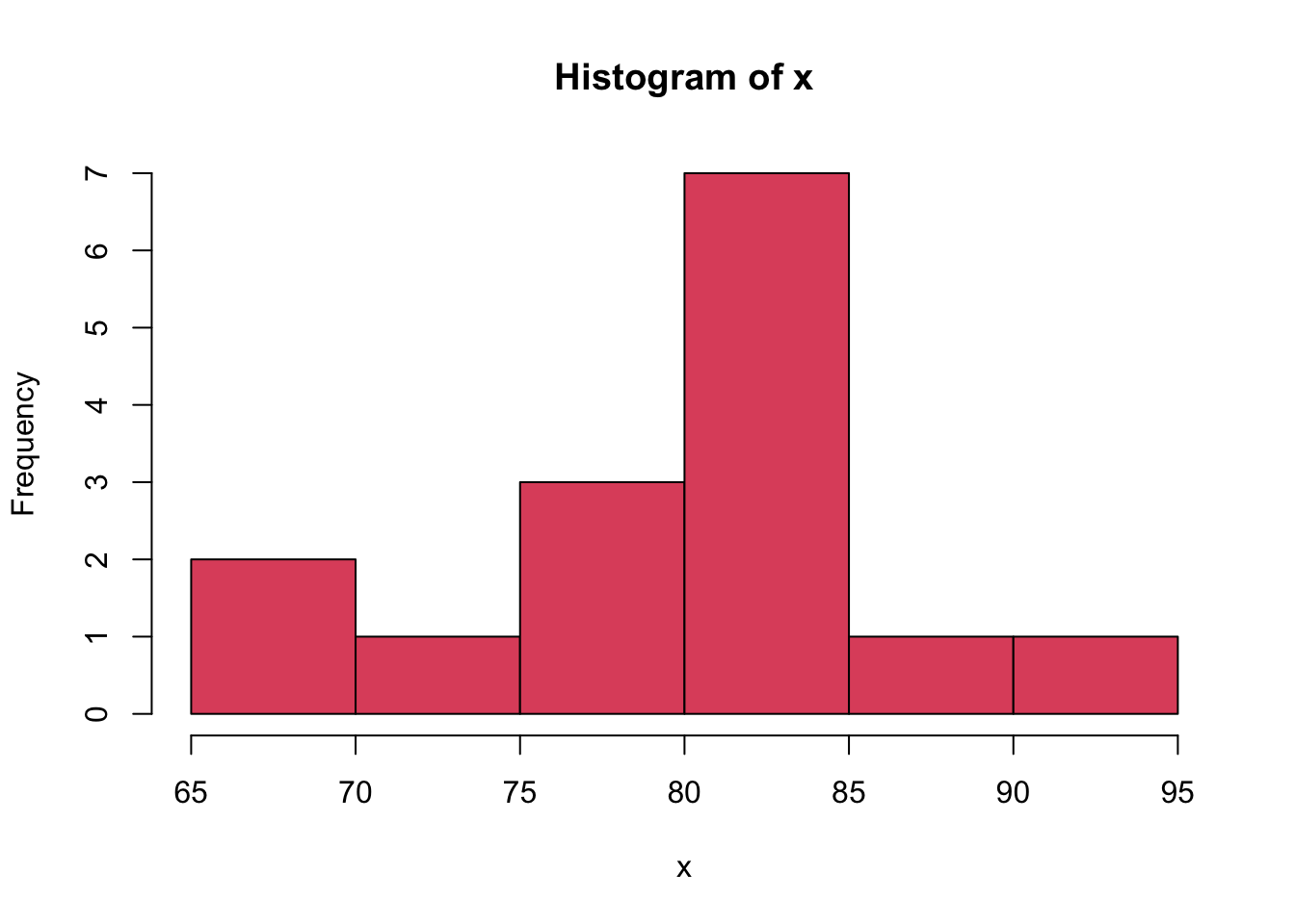
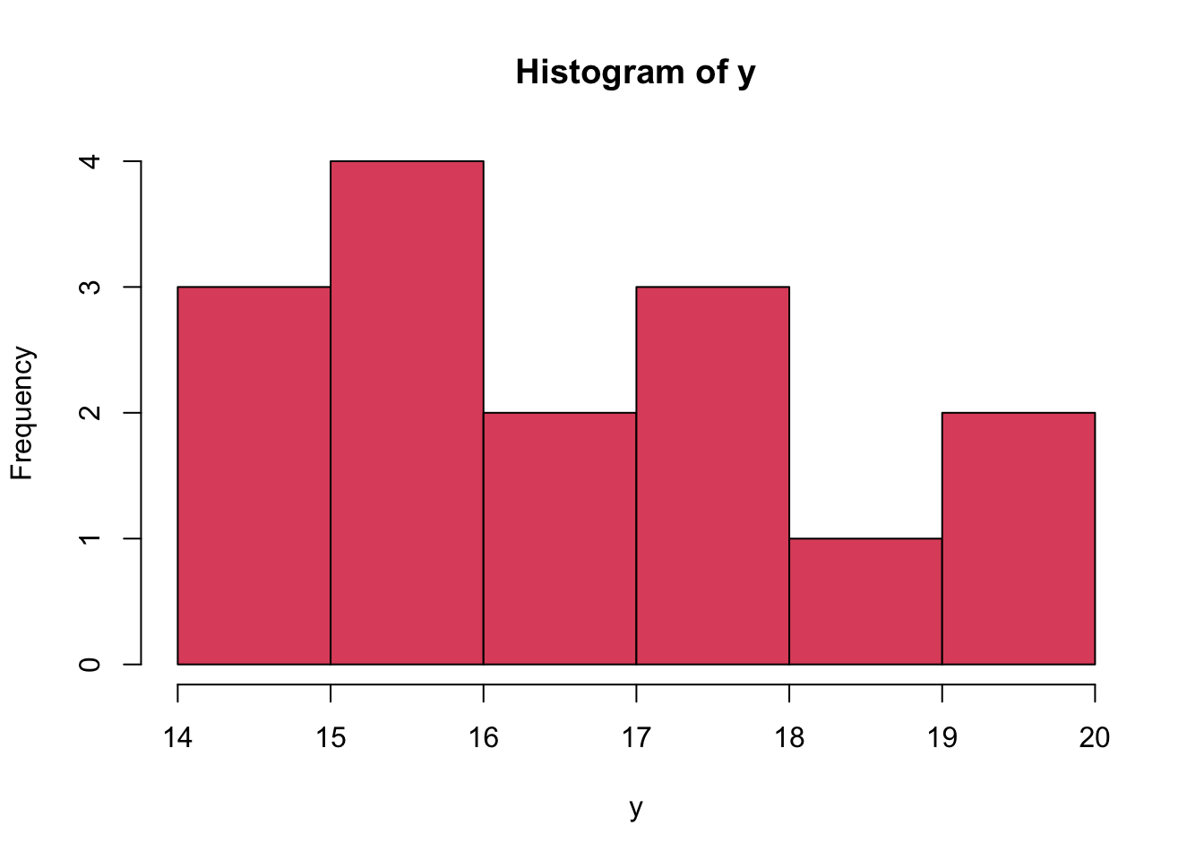
The R module below, shows the Histogram of the monthly births time series in Belgium and the fitted Normal Density. From this illustration it is clear that the time series is not normally distributed because we can identify a bimodal shape in the Histogram (whereas the Normal Distribution is unimodal).
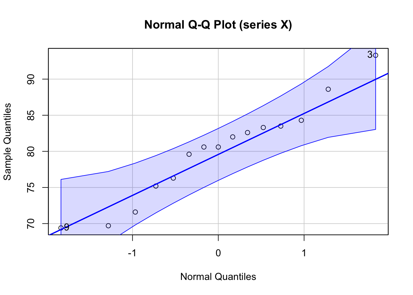
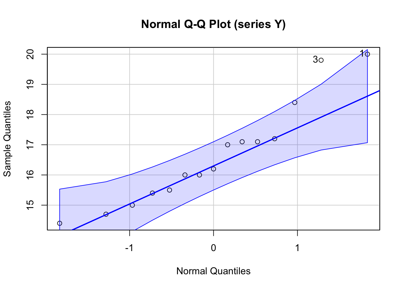
The analysis shows the Normal QQ Plot with confidence intervals. There are many points which fall outside the confidence intervals -- this is an indication that the time series is not normally distributed.
Wilk, M. B., and R. Gnanadesikan. 1968. “Probability Plotting Methods for the Analysis of Data.”Biometrika 55 (1): 1–17. https://doi.org/10.1093/biomet/55.1.1.