141  Leaf Diagnostics for Conditional Inference Trees

141.1 Definition

Leaf diagnostics extend the Conditional Inference Tree workflow (Chapter 140) by evaluating the distribution of a continuous outcome inside each terminal node (leaf).

Instead of reading only leaf means or predicted values, this approach inspects:

• center,
• spread,
• tail behavior,
• and distributional fit quality

within each predicted segment.

141.2 Why This Matters

In regression settings, two leaves can have similar average predictions but very different reliability characteristics. For leaf \(\ell\) with outcome \(Y\):

\[ \mathrm{Var}(Y\mid \ell) \]

may differ strongly across leaves. This is evidence of conditional variance heterogeneity (a heteroskedasticity-like pattern in the prediction structure).

141.3 Practical Workflow

1. Fit a ctree with a continuous outcome.
2. Use terminal nodes as panels.
3. Compare leaf-wise quantiles, variability, and shape diagnostics.
4. Flag leaves with high spread, strong skewness, or heavy tails.
5. Communicate predictions with leaf-specific reliability comments.

For predictive interpretation, this diagnostic should preferably be repeated on a holdout/test sample.

141.4 R Module

141.4.1 Public website

Leaf diagnostics are available through the Conditional EDA app in Tree mode:

• https://shiny.wessa.net/ConditionalEDA

141.4.2 RFC

In RFC, open “Descriptive / Conditional EDA”, switch to Tree mode, select a continuous outcome, and choose exogenous variables for the ctree split structure.

141.5 Example: Regression Leaves for Maximum Heart Rate

The example below models maxheartrateNum using ageNum and thalassemiaLabel, then compares leaf diagnostics panel-by-panel.

Interactive Shiny app (click to load).

Open in new tab

The embedded app uses the heart dataset. The short R example below uses synthetic data so that the same leaf-diagnostics logic can be reproduced directly in code.

141.6 A Minimal R Example of Leaf-Wise Summaries

The same idea can be demonstrated without the app. The code below fits a simple regression tree, records the terminal node for each observation, and then summarizes the response distribution within each leaf.

library(party)

set.seed(321)
n <- 180
age <- sample(25:80, n, replace = TRUE)
risk_group <- factor(sample(c("low", "medium", "high"), n, replace = TRUE,
                            prob = c(0.35, 0.4, 0.25)))

max_rate <- 185 -
  0.55 * age -
  ifelse(risk_group == "high", 18, ifelse(risk_group == "medium", 8, 0)) +
  rnorm(n, sd = ifelse(risk_group == "high", 11, ifelse(risk_group == "medium", 7, 4)))

leaf_data <- data.frame(age = age, risk_group = risk_group, max_rate = max_rate)

leaf_tree <- ctree(
  max_rate ~ age + risk_group,
  data = leaf_data,
  controls = ctree_control(mincriterion = 0.95, minsplit = 20, minbucket = 10)
)

leaf_id <- predict(leaf_tree, type = "node")

leaf_summary <- aggregate(
  max_rate ~ leaf_id,
  data = transform(leaf_data, leaf_id = leaf_id),
  FUN = function(x) c(n = length(x),
                      mean = mean(x),
                      sd = sd(x),
                      q25 = quantile(x, 0.25),
                      median = median(x),
                      q75 = quantile(x, 0.75))
)

leaf_stats <- as.data.frame(leaf_summary$max_rate)
names(leaf_stats) <- c("n", "mean", "sd", "q25", "median", "q75")

leaf_summary <- data.frame(
  leaf = leaf_summary$leaf_id,
  leaf_stats,
  row.names = NULL
)

knitr::kable(
  transform(
    leaf_summary,
    mean = round(mean, 1),
    sd = round(sd, 1),
    q25 = round(q25, 1),
    median = round(median, 1),
    q75 = round(q75, 1)
  ),
  caption = "Leaf-wise summaries for a simple regression tree"
)

Leaf-wise summaries for a simple regression tree

leaf	n	mean	sd	q25	median	q75
5	11	171.5	5.0	168.3	170.3	173.0
6	13	160.1	6.0	157.9	163.1	163.7
9	18	161.7	4.0	159.9	160.4	163.4
10	13	153.9	4.6	151.5	153.8	155.6
11	34	149.5	8.3	141.5	151.1	154.5
12	25	140.8	11.3	132.3	139.8	147.2
15	10	149.7	4.0	146.7	150.8	151.8
16	10	142.5	4.8	139.4	142.7	145.5
19	10	142.5	9.4	138.2	143.5	148.0
20	17	134.7	6.7	131.1	135.8	138.1
21	19	129.5	10.4	121.4	129.1	138.0

boxplot(
  max_rate ~ factor(leaf_id),
  data = transform(leaf_data, leaf_id = leaf_id),
  col = "grey85",
  border = "grey40",
  xlab = "Terminal node",
  ylab = "Maximum heart rate",
  main = "Outcome spread differs across leaves"
)

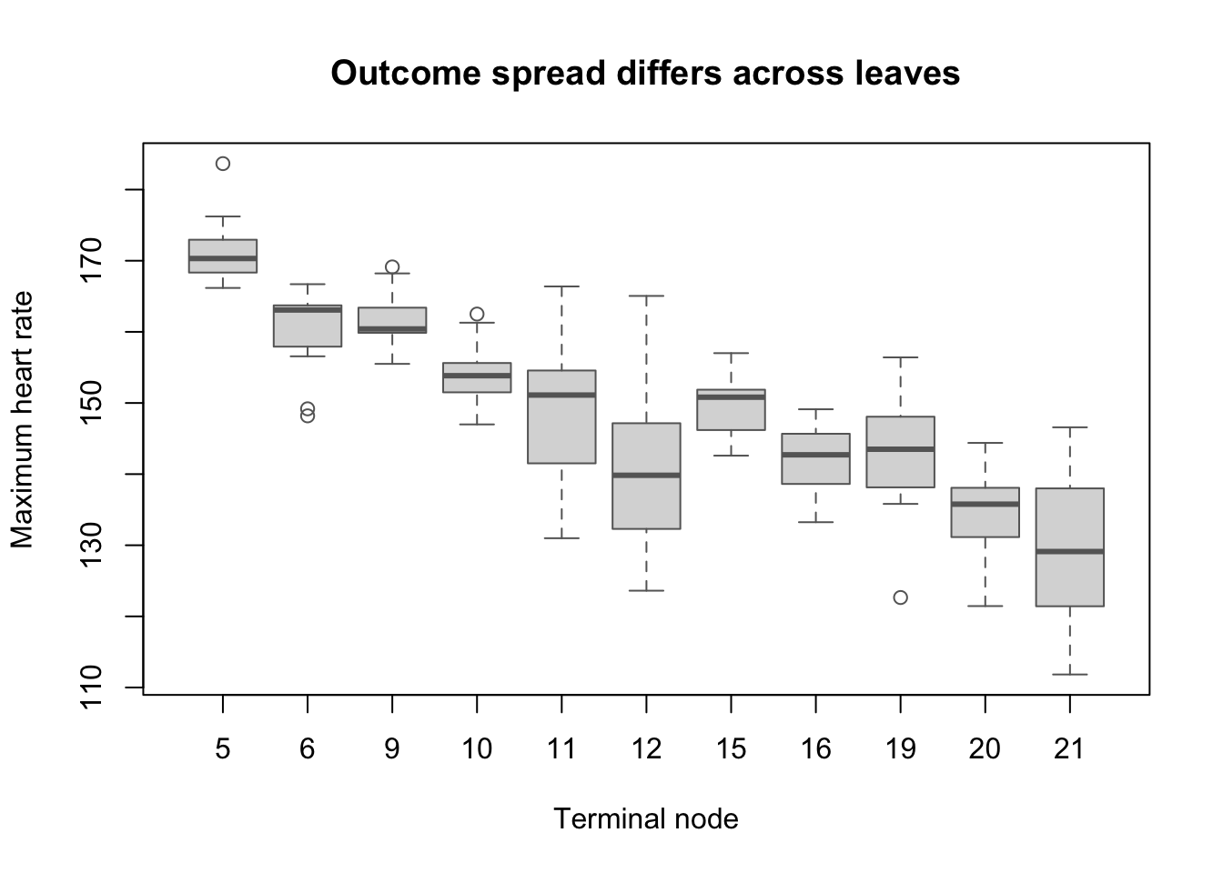
Figure 141.1: Leaf-wise outcome distributions for a regression tree

This is the key idea of leaf diagnostics in one picture: the tree may split the data usefully, but some terminal nodes are still much more variable than others. That difference should appear in how you describe the reliability of predictions.

Detailed interpretation of the synthetic tree example:

1. The terminal nodes separate high- and low-capacity heart-rate segments; the center of max_rate is materially different across leaves.
2. The younger low-risk leaves (for example, nodes 5 and 9) have the highest centers and relatively small spread, so their local predictions are comparatively stable.
3. The medium-risk middle-age leaf (node 11) already shows visibly broader dispersion than the nearby low-risk leaves, even though its center still looks clinically plausible.
4. The high-risk leaves (especially nodes 12 and 21) have the lowest centers and the widest spread, making them the least stable prediction segments in the figure.
5. Interpretation rule: do not treat all leaves as equally reliable. The same tree can contain both well-behaved and weakly-behaved prediction bins.

141.7 Interpreting Leaf Reliability

When comparing leaves:

• low spread + mild asymmetry -> more stable local predictions,
• high spread + heavy tails -> higher uncertainty and lower local reliability,
• severe skew/tails -> consider robust summaries or transformation-sensitive interpretation.

This does not invalidate the tree; it improves how predictions are communicated and where model refinement should focus.

141.8 Pros & Cons

141.8.1 Pros

• adds uncertainty context to leaf predictions,
• improves interpretability of regression trees,
• helps identify segments requiring robust modeling decisions.

141.8.2 Cons

• requires enough observations per leaf,
• can be misread as causal subgroup effects,
• should not replace out-of-sample performance validation.

141.9 Task

Using Tree mode in Conditional EDA:

1. Fit a ctree for a continuous outcome with at least three predictors.
2. Identify one leaf with relatively stable distributional properties and one with unstable properties.
3. Explain how this affects the reliability of predictions for those two segments.