• Descriptive
    • Moments
    • Concentration
    • Central Tendency
    • Variability
    • Stem-and-Leaf Plot
    • Histogram & Frequency Table
    • Data Quality Forensics
    • Conditional EDA
    • Quantiles
    • Kernel Density Estimation
    • Normal QQ Plot
    • Bootstrap Plot

    • Multivariate Descriptive Statistics
  • Distributions
    • Binomial Probabilities
    • Geometric Probabilities
    • Negative Binomial Probabilities
    • Hypergeometric Probabilities
    • Multinomial Probabilities
    • Dirichlet
    • Poisson Probabilities

    • Exponential
    • Gamma
    • Erlang
    • Weibull
    • Rayleigh
    • Maxwell-Boltzmann
    • Lognormal
    • Pareto
    • Inverse Gamma
    • Inverse Chi-Square

    • Beta
    • Power
    • Beta Prime (Inv. Beta)
    • Triangular

    • Normal (area)
    • Logistic
    • Laplace
    • Cauchy (standard)
    • Cauchy (location-scale)
    • Gumbel
    • Fréchet
    • Generalized Extreme Value

    • Normal RNG
    • ML Fitting
    • Tukey Lambda PPCC
    • Box-Cox Normality Plot
    • Noncentral t
    • Noncentral F
    • Sample Correlation r

    • Empirical Tests
  • Hypotheses
    • Theoretical Aspects of Hypothesis Testing
    • Bayesian Inference
    • Minimum Sample Size

    • Empirical Tests
    • Multivariate (pair-wise) Testing
  • Models
    • Manual Model Building
    • Guided Model Building
  • Time Series
    • Time Series Plot
    • Decomposition
    • Exponential Smoothing

    • Blocked Bootstrap Plot
    • Mean Plot
    • (P)ACF
    • VRM
    • Standard Deviation-Mean Plot
    • Spectral Analysis
    • ARIMA

    • Cross Correlation Function
    • Granger Causality
  1. Probability Distributions
  2. 42  Beta Prime Distribution
  • Preface
  • Getting Started
    • 1  Introduction
    • 2  Why Do We Need Innovative Technology?
    • 3  Basic Definitions
    • 4  The Big Picture: Why We Analyze Data
  • Introduction to Probability
    • 5  Definitions of Probability
    • 6  Jeffreys’ axiom system
    • 7  Bayes’ Theorem
    • 8  Sensitivity and Specificity
    • 9  Naive Bayes Classifier
    • 10  Law of Large Numbers

    • 11  Problems
  • Probability Distributions
    • 12  Bernoulli Distribution
    • 13  Binomial Distribution
    • 14  Geometric Distribution
    • 15  Negative Binomial Distribution
    • 16  Hypergeometric Distribution
    • 17  Multinomial Distribution
    • 18  Poisson Distribution

    • 19  Uniform Distribution (Rectangular Distribution)
    • 20  Normal Distribution (Gaussian Distribution)
    • 21  Gaussian Naive Bayes Classifier
    • 22  Chi Distribution
    • 23  Chi-squared Distribution (1 parameter)
    • 24  Chi-squared Distribution (2 parameters)
    • 25  Student t-Distribution
    • 26  Fisher F-Distribution
    • 27  Exponential Distribution
    • 28  Lognormal Distribution
    • 29  Gamma Distribution
    • 30  Beta Distribution
    • 31  Weibull Distribution
    • 32  Pareto Distribution
    • 33  Inverse Gamma Distribution
    • 34  Rayleigh Distribution
    • 35  Erlang Distribution
    • 36  Logistic Distribution
    • 37  Laplace Distribution
    • 38  Gumbel Distribution
    • 39  Cauchy Distribution
    • 40  Triangular Distribution
    • 41  Power Distribution
    • 42  Beta Prime Distribution
    • 43  Sample Correlation Distribution
    • 44  Dirichlet Distribution
    • 45  Generalized Extreme Value (GEV) Distribution
    • 46  Frechet Distribution
    • 47  Noncentral t Distribution
    • 48  Noncentral F Distribution
    • 49  Inverse Chi-Squared Distribution
    • 50  Maxwell-Boltzmann Distribution
    • 51  Distribution Relationship Map

    • 52  Problems
  • Descriptive Statistics & Exploratory Data Analysis
    • 53  Types of Data
    • 54  Datasheets

    • 55  Frequency Plot (Bar Plot)
    • 56  Frequency Table
    • 57  Contingency Table
    • 58  Binomial Classification Metrics
    • 59  Confusion Matrix
    • 60  ROC Analysis

    • 61  Stem-and-Leaf Plot
    • 62  Histogram
    • 63  Data Quality Forensics
    • 64  Quantiles
    • 65  Central Tendency
    • 66  Variability
    • 67  Skewness & Kurtosis
    • 68  Concentration
    • 69  Notched Boxplot
    • 70  Scatterplot
    • 71  Pearson Correlation
    • 72  Rank Correlation
    • 73  Partial Pearson Correlation
    • 74  Simple Linear Regression
    • 75  Moments
    • 76  Quantile-Quantile Plot (QQ Plot)
    • 77  Normal Probability Plot
    • 78  Probability Plot Correlation Coefficient Plot (PPCC Plot)
    • 79  Box-Cox Normality Plot
    • 80  Kernel Density Estimation
    • 81  Bivariate Kernel Density Plot
    • 82  Conditional EDA: Panel Diagnostics
    • 83  Bootstrap Plot (Central Tendency)
    • 84  Survey Scores Rank Order Comparison
    • 85  Cronbach Alpha

    • 86  Equi-distant Time Series
    • 87  Time Series Plot (Run Sequence Plot)
    • 88  Mean Plot
    • 89  Blocked Bootstrap Plot (Central Tendency)
    • 90  Standard Deviation-Mean Plot
    • 91  Variance Reduction Matrix
    • 92  (Partial) Autocorrelation Function
    • 93  Periodogram & Cumulative Periodogram

    • 94  Problems
  • Hypothesis Testing
    • 95  Normal Distributions revisited
    • 96  The Population
    • 97  The Sample
    • 98  The One-Sided Hypothesis Test
    • 99  The Two-Sided Hypothesis Test
    • 100  When to use a one-sided or two-sided test?
    • 101  What if \(\sigma\) is unknown?
    • 102  The Central Limit Theorem (revisited)
    • 103  Statistical Test of the Population Mean with known Variance
    • 104  Statistical Test of the Population Mean with unknown Variance
    • 105  Statistical Test of the Variance
    • 106  Statistical Test of the Population Proportion
    • 107  Statistical Test of the Standard Deviation \(\sigma\)
    • 108  Statistical Test of the difference between Means -- Independent/Unpaired Samples
    • 109  Statistical Test of the difference between Means -- Dependent/Paired Samples
    • 110  Statistical Test of the difference between Variances -- Independent/Unpaired Samples

    • 111  Hypothesis Testing for Research Purposes
    • 112  Decision Thresholds, Alpha, and Confidence Levels
    • 113  Bayesian Inference for Decision-Making
    • 114  One Sample t-Test
    • 115  Skewness & Kurtosis Tests
    • 116  Paired Two Sample t-Test
    • 117  Wilcoxon Signed-Rank Test
    • 118  Unpaired Two Sample t-Test
    • 119  Unpaired Two Sample Welch Test
    • 120  Two One-Sided Tests (TOST) for Equivalence
    • 121  Mann-Whitney U test (Wilcoxon Rank-Sum Test)
    • 122  Bayesian Two Sample Test
    • 123  Median Test based on Notched Boxplots
    • 124  Chi-Squared Tests for Count Data
    • 125  Kolmogorov-Smirnov Test
    • 126  One Way Analysis of Variance (1-way ANOVA)
    • 127  Kruskal-Wallis Test
    • 128  Two Way Analysis of Variance (2-way ANOVA)
    • 129  Repeated Measures ANOVA
    • 130  Friedman Test
    • 131  Testing Correlations
    • 132  A Note on Causality

    • 133  Problems
  • Regression Models
    • 134  Simple Linear Regression Model (SLRM)
    • 135  Multiple Linear Regression Model (MLRM)
    • 136  Logistic Regression
    • 137  Generalized Linear Models
    • 138  Multinomial and Ordinal Logistic Regression
    • 139  Cox Proportional Hazards Regression
    • 140  Conditional Inference Trees
    • 141  Leaf Diagnostics for Conditional Inference Trees
    • 142  Conditional Random Forests
    • 143  Hypothesis Testing with Linear Regression Models (from a Practical Point of View)

    • 144  Problems
  • Introduction to Time Series Analysis
    • 145  Case: the Market of Health and Personal Care Products
    • 146  Decomposition of Time Series
    • 147  Ad hoc Forecasting of Time Series
  • Box-Jenkins Analysis
    • 148  Introduction to Box-Jenkins Analysis
    • 149  Theoretical Concepts
    • 150  Stationarity
    • 151  Identifying ARMA parameters
    • 152  Estimating ARMA Parameters and Residual Diagnostics
    • 153  Forecasting with ARIMA models
    • 154  Intervention Analysis
    • 155  Cross-Correlation Function
    • 156  Transfer Function Noise Models
    • 157  General-to-Specific Modeling
  • Model Building Strategies
    • 158  Introduction to Model Building Strategies
    • 159  Manual Model Building
    • 160  Model Validation
    • 161  Regularization Methods
    • 162  Hyperparameter Optimization Strategies
    • 163  Guided Model Building in Practice
    • 164  Diagnostics, Revision, and Guided Forecasting
    • 165  Leakage, Target Encoding, and Robust Regression
  • References
  • Appendices
    • Appendices
    • A  Method Selection Guide
    • B  Presentations and Teaching Materials
    • C  R Language Concepts for Statistical Computing
    • D  Matrix Algebra
    • E  Standard Normal Table (Gaussian Table)
    • F  Critical values of Student’s \(t\) distribution with \(\nu\) degrees of freedom
    • G  Upper-tail critical values of the \(\chi^2\)-distribution with \(\nu\) degrees of freedom
    • H  Lower-tail critical values of the \(\chi^2\)-distribution with \(\nu\) degrees of freedom

Table of contents

  • 42.1 Probability Density Function
  • 42.2 Purpose
  • 42.3 Distribution Function
  • 42.4 Moment Generating Function
  • 42.5 1st Uncentered Moment
  • 42.6 2nd Uncentered Moment
  • 42.7 3rd Uncentered Moment
  • 42.8 4th Uncentered Moment
  • 42.9 2nd Centered Moment
  • 42.10 3rd Centered Moment
  • 42.11 4th Centered Moment
  • 42.12 Expected Value
  • 42.13 Variance
  • 42.14 Median
  • 42.15 Mode
  • 42.16 Coefficient of Skewness
  • 42.17 Coefficient of Kurtosis
  • 42.18 Parameter Estimation
  • 42.19 R Module
    • 42.19.1 RFC
    • 42.19.2 Direct app link
    • 42.19.3 R Code
  • 42.20 Example
  • 42.21 Random Number Generator
  • 42.22 Property 1: Beta Transformation
  • 42.23 Property 2: F Distribution Relationship
  • 42.24 Property 3: Lomax (Shifted Pareto) Special Case
  • 42.25 Related Distributions 1: Beta Distribution
  • 42.26 Related Distributions 2: F Distribution
  • 42.27 Related Distributions 3: Pareto Distribution
  1. Probability Distributions
  2. 42  Beta Prime Distribution

42  Beta Prime Distribution

The Beta Prime distribution — also called the Inverted Beta or Beta Distribution of the Second Kind — extends the Beta distribution to the positive half-line. While the Beta models a proportion bounded to \([0,1]\), the Beta Prime models a positive ratio with no upper bound, arising naturally in Bayesian hierarchical models and as a distribution for odds ratios.

Formally, the random variate \(X\) defined for the range \(X > 0\), is said to have a Beta Prime Distribution (i.e. \(X \sim \text{BetaPrime}(\alpha, \beta, \theta)\)) with shape parameters \(\alpha > 0\) and \(\beta > 0\), and scale parameter \(\theta > 0\). If \(Y \sim \text{Beta}(\alpha, \beta)\) then \(\theta Y/(1-Y) \sim \text{BetaPrime}(\alpha, \beta, \theta)\).

42.1 Probability Density Function

\[ f(x) = \frac{(x/\theta)^{\alpha-1}(1+x/\theta)^{-\alpha-\beta}}{\theta\,\text{B}(\alpha,\beta)}, \quad x > 0 \]

where \(\text{B}(\alpha, \beta) = \Gamma(\alpha)\Gamma(\beta)/\Gamma(\alpha+\beta)\).

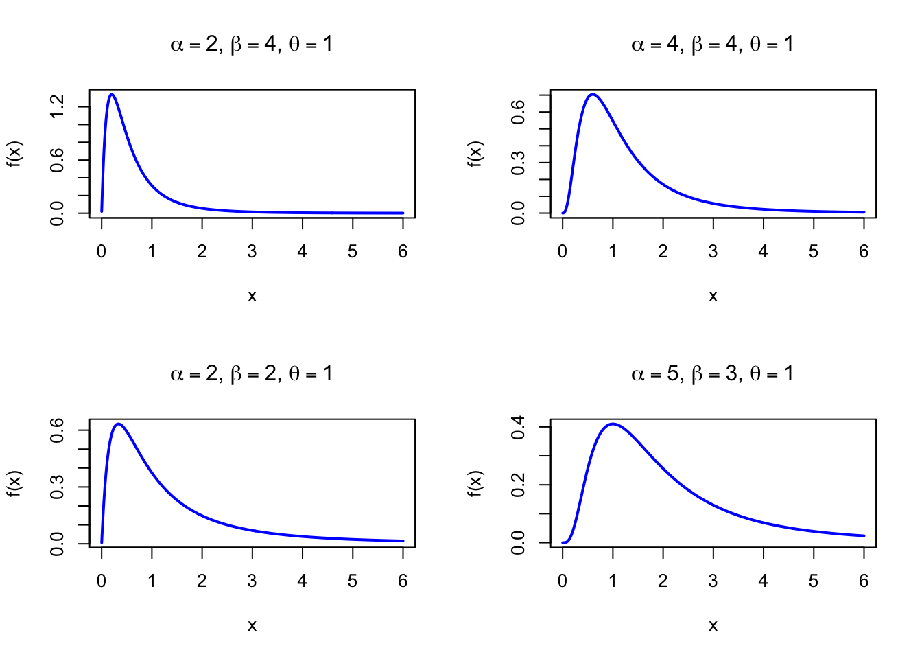
The figure below shows examples of the Beta Prime Probability Density Function for different parameter combinations with \(\theta = 1\).

Code
dbetaprime <- function(x, alpha, beta, theta = 1) {
  ifelse(x > 0,
         (x/theta)^(alpha-1) * (1 + x/theta)^(-alpha-beta) /
           (theta * beta(alpha, beta)),
         0)
}

par(mfrow = c(2, 2))
x <- seq(0.001, 6, length = 500)

plot(x, dbetaprime(x, 2, 4, 1), type = "l", lwd = 2, col = "blue",
     xlab = "x", ylab = "f(x)", main = expression(paste(alpha==2, ", ", beta==4, ", ", theta==1)))

plot(x, dbetaprime(x, 4, 4, 1), type = "l", lwd = 2, col = "blue",
     xlab = "x", ylab = "f(x)", main = expression(paste(alpha==4, ", ", beta==4, ", ", theta==1)))

plot(x, dbetaprime(x, 2, 2, 1), type = "l", lwd = 2, col = "blue",
     xlab = "x", ylab = "f(x)", main = expression(paste(alpha==2, ", ", beta==2, ", ", theta==1)))

plot(x, dbetaprime(x, 5, 3, 1), type = "l", lwd = 2, col = "blue",
     xlab = "x", ylab = "f(x)", main = expression(paste(alpha==5, ", ", beta==3, ", ", theta==1)))

par(mfrow = c(1, 1))
Figure 42.1: Beta Prime Probability Density Function for various parameter combinations (scale = 1)

42.2 Purpose

The Beta Prime distribution models positive, right-skewed quantities for which the support extends to infinity but is bounded below by zero. It generalizes the Beta distribution to the full positive half-line via an odds-ratio transformation and arises naturally in Bayesian inference as a marginal distribution. Common applications include:

  • Odds ratios in clinical trials and epidemiology (positive, unbounded, right-skewed)
  • Bayesian hierarchical models: scale parameter priors with heavy right tails
  • Variance-ratio statistics: the F distribution is a scaled Beta Prime
  • Financial loss ratios: claim amount relative to policy limit
  • Reliability and survival: ratio of component strengths or lifetimes

Relation to the discrete setting. The Beta Prime arises in the same way as the Negative Binomial for count data: just as Poisson-Gamma mixture yields the Negative Binomial, a Beta-Prime-type distribution emerges as the marginal of Poisson-Gamma hierarchies for rates. Both generalize their simpler counterparts to handle overdispersion.

42.3 Distribution Function

\[ F(x) = I_{x/(x+\theta)}(\alpha, \beta) \]

where \(I_u(\alpha, \beta)\) is the regularized incomplete beta function. In R: pbeta(x/(x+theta), shape1 = alpha, shape2 = beta).

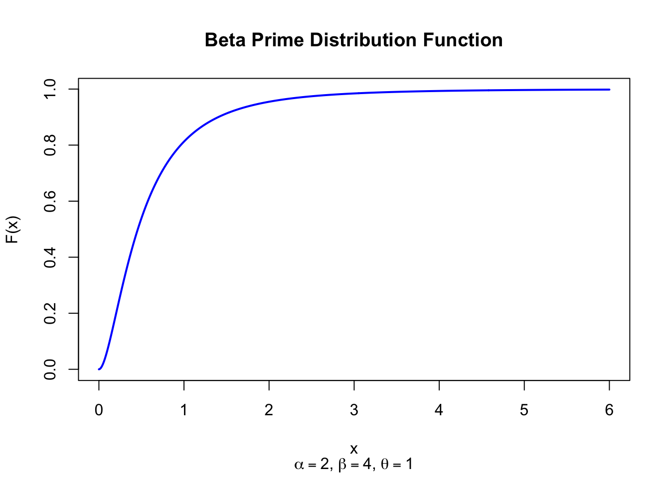
The figure below shows the Beta Prime Distribution Function for \(\alpha = 2\), \(\beta = 4\), \(\theta = 1\).

Code
pbetaprime <- function(x, alpha, beta, theta = 1) {
  ifelse(x > 0, pbeta(x / (x + theta), shape1 = alpha, shape2 = beta), 0)
}

x <- seq(0, 6, length = 500)
plot(x, pbetaprime(x, 2, 4, 1), type = "l", lwd = 2, col = "blue",
     xlab = "x", ylab = "F(x)", main = "Beta Prime Distribution Function",
     sub = expression(paste(alpha==2, ", ", beta==4, ", ", theta==1)))
Figure 42.2: Beta Prime Distribution Function (alpha = 2, beta = 4, scale = 1)

42.4 Moment Generating Function

The moment generating function does not exist for \(t > 0\) due to the heavy right tail.

42.5 1st Uncentered Moment

\[ \mu_1' = \frac{\theta\,\alpha}{\beta - 1}, \quad \beta > 1 \]

42.6 2nd Uncentered Moment

\[ \mu_2' = \frac{\theta^2\,\alpha(\alpha+1)}{(\beta-1)(\beta-2)}, \quad \beta > 2 \]

42.7 3rd Uncentered Moment

\[ \mu_3' = \frac{\theta^3\,\alpha(\alpha+1)(\alpha+2)}{(\beta-1)(\beta-2)(\beta-3)}, \quad \beta > 3 \]

42.8 4th Uncentered Moment

\[ \mu_4' = \frac{\theta^4\,\alpha(\alpha+1)(\alpha+2)(\alpha+3)}{(\beta-1)(\beta-2)(\beta-3)(\beta-4)}, \quad \beta > 4 \]

In general: \(\mu_n' = \theta^n\,\text{B}(\alpha+n,\,\beta-n)/\text{B}(\alpha,\beta)\) for \(n < \beta\).

42.9 2nd Centered Moment

\[ \mu_2 = \frac{\theta^2\,\alpha(\alpha+\beta-1)}{(\beta-1)^2(\beta-2)}, \quad \beta > 2 \]

42.10 3rd Centered Moment

Obtained by expanding from raw moments; requires \(\beta > 3\).

42.11 4th Centered Moment

Obtained by expanding from raw moments; requires \(\beta > 4\).

42.12 Expected Value

\[ \text{E}(X) = \frac{\theta\,\alpha}{\beta - 1}, \quad \beta > 1 \]

42.13 Variance

\[ \text{V}(X) = \frac{\theta^2\,\alpha(\alpha+\beta-1)}{(\beta-1)^2(\beta-2)}, \quad \beta > 2 \]

42.14 Median

The median has no closed form and is computed numerically via qbeta.

42.15 Mode

\[ \text{Mo}(X) = \begin{cases} \theta\,\dfrac{\alpha-1}{\beta+1} & \alpha > 1 \\[4pt] 0 & \alpha \leq 1 \end{cases} \]

42.16 Coefficient of Skewness

\[ g_1 = \frac{2(2\alpha+\beta-1)}{\beta-3}\sqrt{\frac{\beta-2}{\alpha(\alpha+\beta-1)}}, \quad \beta > 3 \]

42.17 Coefficient of Kurtosis

\[ g_2 = \frac{3(\beta-2)\bigl(\alpha^2\beta + 5\alpha^2 + \alpha\beta^2 + 4\alpha\beta - 5\alpha + 2\beta^2 - 4\beta + 2\bigr)}{\alpha(\beta-4)(\beta-3)(\alpha+\beta-1)}, \quad \beta > 4 \]

The kurtosis is always greater than 3 for valid parameter values.

42.18 Parameter Estimation

Maximum likelihood estimation is numerical. Method-of-moments provides starting values from the mean and variance:

set.seed(42)
alpha_true <- 2; beta_true <- 4; theta_true <- 1

# Simulate BetaPrime via Beta transformation
y <- rbeta(100, shape1 = alpha_true, shape2 = beta_true)
x_obs <- theta_true * y / (1 - y)

# Summary statistics
cat("Sample mean:", round(mean(x_obs), 4), "\n")
cat("Theoretical mean:", theta_true * alpha_true / (beta_true - 1), "\n")
cat("Sample var:", round(var(x_obs), 4), "\n")
cat("Theoretical var:",
    theta_true^2 * alpha_true * (alpha_true + beta_true - 1) /
    ((beta_true - 1)^2 * (beta_true - 2)), "\n")
Sample mean: 0.6892 
Theoretical mean: 0.6666667 
Sample var: 0.5095 
Theoretical var: 0.5555556 

42.19 R Module

42.19.1 RFC

The Beta Prime Distribution module is available in RFC under the menu “Distributions / Beta Prime Distribution”.

42.19.2 Direct app link

  • https://shiny.wessa.net/invbeta/

42.19.3 R Code

The following code demonstrates Beta Prime probability calculations:

alpha <- 2; beta <- 4; theta <- 1

pbetaprime <- function(x, alpha, beta, theta = 1) {
  ifelse(x > 0, pbeta(x / (x + theta), shape1 = alpha, shape2 = beta), 0)
}

# P(X <= 1)
pbetaprime(1, alpha, beta, theta)

# Mean and mode
cat("Mean:", theta * alpha / (beta - 1), "\n")
cat("Mode:", theta * (alpha - 1) / (beta + 1), "\n")
[1] 0.8125
Mean: 0.6666667 
Mode: 0.2 

42.20 Example

An odds ratio for a treatment effect is modeled as \(X \sim \text{BetaPrime}(\alpha = 2, \beta = 4, \theta = 1)\). The mean odds ratio is \(\alpha/(\beta-1) = 2/3\) and the mode is \((\alpha-1)/(\beta+1) = 1/5\).

alpha <- 2; beta <- 4; theta <- 1

pbetaprime <- function(x, alpha, beta, theta = 1) {
  ifelse(x > 0, pbeta(x / (x + theta), shape1 = alpha, shape2 = beta), 0)
}

# P(odds ratio <= 1)
cat("P(odds ratio <= 1):", round(pbetaprime(1, alpha, beta, theta), 4), "\n")

# Mean and mode
cat("Mean odds ratio:", theta * alpha / (beta - 1), "\n")
cat("Mode:", theta * (alpha - 1) / (beta + 1), "\n")
P(odds ratio <= 1): 0.8125 
Mean odds ratio: 0.6666667 
Mode: 0.2 
Interactive Shiny app (click to load).
Open in new tab

42.21 Random Number Generator

Beta Prime random variates are generated via the Beta transformation:

\[ \text{If } Y \sim \text{Beta}(\alpha, \beta) \text{ then } X = \frac{\theta Y}{1-Y} \sim \text{BetaPrime}(\alpha, \beta, \theta) \]

set.seed(123)
n <- 1000; alpha <- 2; beta <- 4; theta <- 1

# Generate via Beta transformation
y <- rbeta(n, shape1 = alpha, shape2 = beta)
x_sim <- theta * y / (1 - y)

cat("Simulated mean:", round(mean(x_sim), 4), "\n")
cat("Theoretical mean:", theta * alpha / (beta - 1), "\n")
Simulated mean: 0.6751 
Theoretical mean: 0.6666667 
Interactive Shiny app (click to load).
Open in new tab

42.22 Property 1: Beta Transformation

If \(Y \sim \text{Beta}(\alpha, \beta)\) then \(\theta Y/(1-Y) \sim \text{BetaPrime}(\alpha, \beta, \theta)\). This is the defining property and provides the simplest interpretation: the Beta Prime models odds-ratio-type quantities derived from bounded Beta variates (see Chapter 30).

42.23 Property 2: F Distribution Relationship

If \(X \sim F(2\alpha, 2\beta)\) (Fisher-Snedecor F), then \((\alpha/\beta) X \sim \text{BetaPrime}(\alpha, \beta, 1)\). This means the F distribution is a scaled Beta Prime, and tables of the F distribution implicitly cover the Beta Prime (see Chapter 26).

42.24 Property 3: Lomax (Shifted Pareto) Special Case

When \(\alpha = 1\): \(\text{BetaPrime}(1, \beta, \theta)\) is the Lomax distribution (also known as the shifted Pareto or Pareto Type II). See Chapter 32.

42.25 Related Distributions 1: Beta Distribution

The Beta Prime arises from the Beta via the odds-ratio transformation (see Chapter 30).

42.26 Related Distributions 2: F Distribution

The F distribution is a scaled Beta Prime with integer shape parameters (see Chapter 26).

42.27 Related Distributions 3: Pareto Distribution

The Lomax distribution BetaPrime\((1, \beta, \theta)\) is a shifted Pareto distribution (see Chapter 32).

41  Power Distribution
43  Sample Correlation Distribution

© 2026 Patrick Wessa. Provided as-is, without warranty.

Feedback: e-mail | Anonymous contributions: click to copy (Sats) | click to copy (XMR)

Cookie Preferences