31  Weibull Distribution

The Weibull distribution is the workhorse of reliability engineering and survival analysis. By tuning a single shape parameter, it can model failure rates that increase, decrease, or remain constant over time — making it far more flexible than the Exponential distribution.

Formally, the random variate \(X\) defined for the range \(X \in [0, \infty)\), is said to have a Weibull Distribution (i.e. \(X \sim \text{Weibull}(k, \lambda)\)) with shape parameter \(k > 0\) and scale parameter \(\lambda > 0\). In R, these parameters are named shape (\(= k\)) and scale (\(= \lambda\)).

31.1 Probability Density Function

\[ f(x) = \frac{k}{\lambda}\left(\frac{x}{\lambda}\right)^{k-1}\exp\!\left(-\left(\frac{x}{\lambda}\right)^k\right), \quad x \geq 0 \]

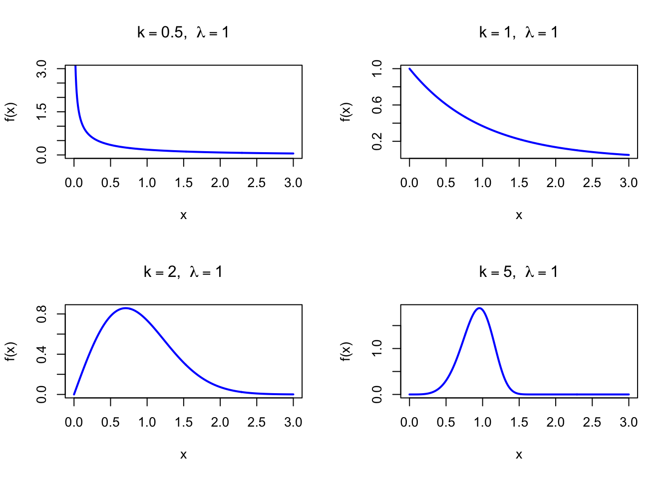
The figure below shows examples of the Weibull Probability Density Function for different shape values with \(\lambda = 1\).

par(mfrow = c(2, 2))
x <- seq(0, 3, length = 500)

plot(x, dweibull(x, shape = 0.5, scale = 1), type = "l", lwd = 2, col = "blue",
     xlab = "x", ylab = "f(x)", main = expression(paste(k == 0.5, ",  ", lambda == 1)),
     ylim = c(0, 3))

plot(x, dweibull(x, shape = 1, scale = 1), type = "l", lwd = 2, col = "blue",
     xlab = "x", ylab = "f(x)", main = expression(paste(k == 1, ",  ", lambda == 1)))

plot(x, dweibull(x, shape = 2, scale = 1), type = "l", lwd = 2, col = "blue",
     xlab = "x", ylab = "f(x)", main = expression(paste(k == 2, ",  ", lambda == 1)))

plot(x, dweibull(x, shape = 5, scale = 1), type = "l", lwd = 2, col = "blue",
     xlab = "x", ylab = "f(x)", main = expression(paste(k == 5, ",  ", lambda == 1)))

par(mfrow = c(1, 1))

Figure 31.1: Weibull Probability Density Function for various shape values (scale = 1)

31.2 Purpose

The Weibull distribution models the lifetime of components and systems when the hazard rate (instantaneous failure rate) is not constant. By varying the shape parameter \(k\), it can capture early-life failures (\(k < 1\)), random failures (\(k = 1\), identical to the Exponential), or wear-out failures (\(k > 1\)). Common applications include:

• Reliability engineering: time to failure of mechanical and electronic components
• Survival analysis: patient survival times, where hazard may change over time
• Wind energy: wind speed distributions for turbine siting and energy estimation
• Materials science: fatigue life and fracture strength distributions
• Extreme-value analysis: minimum strength and maximum stress models

Relation to the discrete setting. The Weibull distribution extends the Exponential (continuous Geometric analog). For \(k = 1\): constant hazard rate corresponds to Geometric memorylessness. For \(k \neq 1\), the Discrete Weibull distribution is the closest analog (not covered here).

31.3 Distribution Function

\[ F(x) = 1 - \exp\!\left(-\left(\frac{x}{\lambda}\right)^k\right), \quad x \geq 0 \]

The figure below shows the Weibull Distribution Function for \(k = 2\) and \(\lambda = 1\).

x <- seq(0, 3, length = 500)
plot(x, pweibull(x, shape = 2, scale = 1), type = "l", lwd = 2, col = "blue",
     xlab = "x", ylab = "F(x)", main = "Weibull Distribution Function",
     sub = expression(paste(k == 2, ",  ", lambda == 1)))

Figure 31.2: Weibull Distribution Function (shape = 2, scale = 1)

31.4 Moment Generating Function

The moment generating function of the Weibull distribution does not have a closed form in general. Raw moments are given by:

\[ \mu_n' = \lambda^n\,\Gamma\!\left(1 + \frac{n}{k}\right) \]

31.5 1st Uncentered Moment

\[ \mu_1' = \lambda\,\Gamma\!\left(1 + \frac{1}{k}\right) \]

31.6 2nd Uncentered Moment

\[ \mu_2' = \lambda^2\,\Gamma\!\left(1 + \frac{2}{k}\right) \]

31.7 3rd Uncentered Moment

\[ \mu_3' = \lambda^3\,\Gamma\!\left(1 + \frac{3}{k}\right) \]

31.8 4th Uncentered Moment

\[ \mu_4' = \lambda^4\,\Gamma\!\left(1 + \frac{4}{k}\right) \]

31.9 2nd Centered Moment

\[ \mu_2 = \lambda^2\!\left[\Gamma\!\left(1+\frac{2}{k}\right) - \Gamma\!\left(1+\frac{1}{k}\right)^2\right] \]

31.10 3rd Centered Moment

\[ \mu_3 = \lambda^3\!\left[\Gamma\!\left(1+\frac{3}{k}\right) - 3\,\Gamma\!\left(1+\frac{2}{k}\right)\Gamma\!\left(1+\frac{1}{k}\right) + 2\,\Gamma\!\left(1+\frac{1}{k}\right)^3\right] \]

31.11 4th Centered Moment

\[ \mu_4 = \lambda^4\!\left[\Gamma\!\left(1+\frac{4}{k}\right) - 4\,\Gamma\!\left(1+\frac{3}{k}\right)\Gamma\!\left(1+\frac{1}{k}\right) + 6\,\Gamma\!\left(1+\frac{2}{k}\right)\Gamma\!\left(1+\frac{1}{k}\right)^2 - 3\,\Gamma\!\left(1+\frac{1}{k}\right)^4\right] \]

31.12 Expected Value

\[ \text{E}(X) = \lambda\,\Gamma\!\left(1 + \frac{1}{k}\right) \]

31.13 Variance

\[ \text{V}(X) = \lambda^2\!\left[\Gamma\!\left(1+\frac{2}{k}\right) - \Gamma\!\left(1+\frac{1}{k}\right)^2\right] \]

31.14 Median

\[ \text{Med}(X) = \lambda\,(\ln 2)^{1/k} \]

31.15 Mode

\[ \text{Mo}(X) = \lambda\left(\frac{k-1}{k}\right)^{1/k} \text{ for } k > 1; \quad 0 \text{ for } k \leq 1 \]

31.16 Coefficient of Skewness

\[ g_1 = \frac{\mu_3}{\mu_2^{3/2}} \]

where \(\mu_2\) and \(\mu_3\) are the centered moments given above. For \(k = 1\) (Exponential), \(g_1 = 2\).

31.17 Coefficient of Kurtosis

\[ g_2 = \frac{\mu_4}{\mu_2^2} \]

where \(\mu_2\) and \(\mu_4\) are the centered moments given above. For \(k = 1\) (Exponential), \(g_2 = 9\).

31.18 Parameter Estimation

Maximum likelihood estimates are obtained numerically. A convenient starting point uses method-of-moments estimates. In R:

library(MASS)

# Example: bearing lifetime data (hours)
set.seed(42)
lifetimes <- rweibull(50, shape = 2, scale = 5)

# Maximum likelihood estimation
fit <- fitdistr(lifetimes, "weibull")
print(fit)

     shape       scale  
  1.5671275   4.2320164 
 (0.1685372) (0.4038208)

31.19 R Module

31.19.1 RFC

The Weibull Distribution module is available in RFC under the menu “Distributions / Weibull Distribution”.

31.19.2 Direct app link

• https://shiny.wessa.net/weibull/

31.19.3 R Code

The following code demonstrates Weibull probability calculations:

k <- 2; lambda <- 5

# Probability density function: f(x)
dweibull(x = 4, shape = k, scale = lambda)

# Distribution function: P(X <= x)
pweibull(q = 4, shape = k, scale = lambda)

# Quantile function: median lifetime
qweibull(p = 0.5, shape = k, scale = lambda)

# Generate random Weibull numbers
set.seed(42)
rweibull(n = 10, shape = k, scale = lambda)

[1] 0.1687336
[1] 0.4727076
[1] 4.162773
 [1] 1.492005 1.274672 5.593022 2.155171 3.330028 4.048662 2.764625 7.079819
 [9] 3.240690 2.955781

31.20 Example

A bearing manufacturer models component lifetime (in hours) as \(X \sim \text{Weibull}(k = 2, \lambda = 5)\). The shape \(k = 2 > 1\) indicates wear-out failure: the hazard rate increases over time. The mean lifetime is \(5\,\Gamma(1.5) \approx 4.43\) hours.

k <- 2; lambda <- 5

# P(X <= 4): probability of failure within 4 hours
cat("P(fails within 4 h):", pweibull(4, shape = k, scale = lambda), "\n")

# Median lifetime
cat("Median lifetime (h):", qweibull(0.5, shape = k, scale = lambda), "\n")

# Mean lifetime
cat("Mean lifetime (h):", lambda * gamma(1 + 1/k), "\n")

P(fails within 4 h): 0.4727076 
Median lifetime (h): 4.162773 
Mean lifetime (h): 4.431135 

Interactive Shiny app (click to load).

Open in new tab

31.21 Random Number Generator

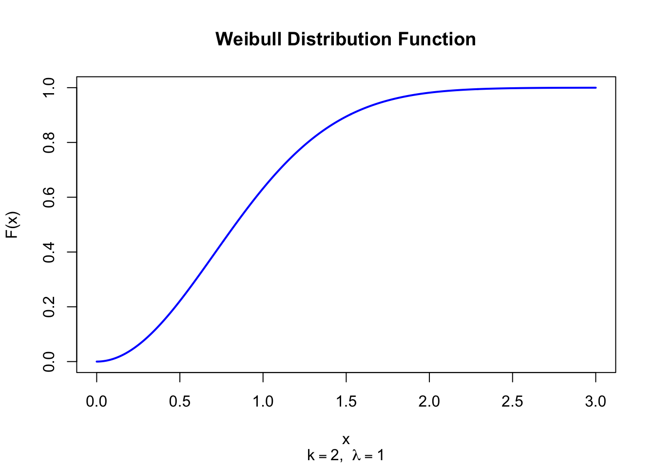
Weibull random variates are generated via the inverse-CDF method. Since \(F(x) = 1 - \exp(-(x/\lambda)^k)\), setting \(U = F(X)\) and solving for \(X\) gives:

\[ X = \lambda\,(-\ln U)^{1/k} \sim \text{Weibull}(k, \lambda) \quad \text{when } U \sim \text{U}(0,1) \]

set.seed(123)
n <- 1000
k <- 2; lambda <- 5

# Inverse-transform method
u <- runif(n)
x_inv <- lambda * (-log(u))^(1/k)

cat("Inverse-transform: mean =", round(mean(x_inv), 4),
    "  var =", round(var(x_inv), 4), "\n")
cat("Theoretical mean:", lambda * gamma(1 + 1/k), "\n")
cat("Theoretical var:", lambda^2 * (gamma(1 + 2/k) - gamma(1 + 1/k)^2), "\n")

Inverse-transform: mean = 4.451   var = 5.3529 
Theoretical mean: 4.431135 
Theoretical var: 5.365046 

Interactive Shiny app (click to load).

Open in new tab

31.22 Property 1: Generalizes the Exponential Distribution

When \(k = 1\), the Weibull reduces to the Exponential distribution with rate \(1/\lambda\):

\[ \text{Weibull}(1, \lambda) = \text{Exp}(1/\lambda) \]

See Chapter 27.

31.23 Property 2: Reduces to the Rayleigh Distribution

When \(k = 2\), the Weibull reduces to the Rayleigh distribution with parameter \(\sigma = \lambda/\sqrt{2}\):

\[ \text{Weibull}(2, \lambda) = \text{Rayleigh}(\lambda/\sqrt{2}) \]

See Chapter 34.

31.24 Property 3: Hazard Rate

The hazard (failure) rate of the Weibull distribution is:

\[ h(x) = \frac{f(x)}{1 - F(x)} = \frac{k}{\lambda}\left(\frac{x}{\lambda}\right)^{k-1} \]

This rate is increasing for \(k > 1\) (wear-out failures), constant for \(k = 1\) (random failures), and decreasing for \(k < 1\) (infant mortality). The two-parameter Weibull therefore models monotone hazards; bathtub-shaped hazards require extended, piecewise, or mixture models.

31.25 Related Distributions 1: Exponential Distribution

The Exponential distribution is the special case \(k = 1\) of the Weibull (see Chapter 27).

31.26 Related Distributions 2: Rayleigh Distribution

The Rayleigh distribution is the special case \(k = 2\) of the Weibull (see Chapter 34).

31.27 Related Distributions 3: Gumbel Distribution

If \(X \sim \text{Weibull}(k, \lambda)\) then \(\ln\!\left((X/\lambda)^k\right) \sim \text{Gumbel}(0, 1)\) (minimum Gumbel), while \(-\ln\!\left((X/\lambda)^k\right)\) follows the maximum Gumbel. See Chapter 38.

31.28 Related Distributions 4: GEV Distribution

The Weibull minimum distribution appears as the GEV Type III extreme-value distribution when \(\xi < 0\): \(\text{GEV}(\mu, \sigma, \xi < 0)\) has a finite upper endpoint and is related to the reversed Weibull (see Chapter 45).

31.29 Related Distributions 5: Fréchet Distribution

The Fréchet distribution is the GEV Type II extreme-value distribution (\(\xi > 0\)), governing the maximum of heavy-tailed parent distributions such as Pareto. The Weibull and Fréchet represent opposite tails of the GEV family: light-tailed (finite endpoint) versus heavy-tailed (polynomial decay) (see Chapter 46).