74  Simple Linear Regression

74.1 General Simple Linear Model

The General Simple Linear Model predicts the endogenous variable \(y\) by the exogenous variable \(x\). The mathematical relationship of this model is defined as a linear equation:

\[ y_i = \beta_0 + \beta_1 x_i + \epsilon_i \]

for \(i = 1, 2, …, n\).

74.1.1 Ordinary Least Squares (OLS) Estimators

The OLS approach (Legendre 1805) estimates \(\beta_0\) and \(\beta_1\) by minimizing the sum of squared residuals:

\[ SSE = \sum_{i=1}^{n} \left(y_i - \hat{\beta}_0 - \hat{\beta}_1 x_i \right)^2 \]

The resulting estimators are

\[ \hat{\beta}_1 = \frac{\sum_{i=1}^{n} (x_i-\bar{x})(y_i-\bar{y})}{\sum_{i=1}^{n}(x_i-\bar{x})^2} \]

and

\[ \hat{\beta}_0 = \bar{y} - \hat{\beta}_1 \bar{x} \]

The fitted values and residuals are then

\[ \hat{y}_i = \hat{\beta}_0 + \hat{\beta}_1 x_i, \qquad \hat{\epsilon}_i = y_i - \hat{y}_i \]

Note: when reporting residual variance in simple regression, software typically applies a degrees-of-freedom correction and divides by \((n-2)\).

74.1.2 Model Assumption 1

The prediction errors \(\epsilon\) have an expectation of zero:

\[ \text{E}(\epsilon_i) = 0 \]

for \(i = 1, 2, …, n\).

This implies that the errors are on average zero (i.e. negative errors are compensated by positive errors). This assumption is basically true when the model specification is true. In other words, if the model has been correctly specified then \(\forall i = 1, 2, …,n:\) E\((y_i) = \beta_0 + \beta_1 x_i\) which implies that E\((\epsilon_i) = 0\).

74.1.3 Model Assumption 2

\(\forall i,j = 1, 2, …, n \text{ and } i = j:\)

\[ \text{E}\left(\epsilon_i \epsilon_j\right) = \text{C}\left( \epsilon_i \epsilon_j \right) = \text{V}\left( \epsilon_i \right) = \text{V}\left( \epsilon_j \right) = \sigma^2 \]

\(\forall i,j = 1, 2, …, n \text{ and } i \neq j:\)

\[ \text{E}\left( \epsilon_i \epsilon_j \right) = \text{C} \left( \epsilon_i \epsilon_j \right) = 0 \]

This assumption implies that:

• The prediction errors are mutually uncorrelated (i.e. zero covariance).
• The prediction errors have a fixed Variance \(\sigma^2\).

74.1.4 Model Assumption 3

The vector of prediction errors has a Normal Distribution with zero mean and fixed, diagonal covariance:

\[ \epsilon \sim \text{N}\left( 0, \sigma^2 I \right) \]

Note: the mean and covariance structure is actually a consequence of assumptions 1 & 2. The normality of prediction errors is an additional modeling assumption used for exact small-sample inference (see Hypothesis Testing). It is not a direct consequence of the Central Limit Theorem.

74.2 Horizontal axis

The horizontal axis shows the values of the exogenous variable \(x\).

74.3 Vertical axis

The vertical axis shows the values of the endogenous variable \(y\).

74.4 R Module

74.4.1 Public website

The Simple Linear Regression module is available on the public website:

• https://compute.wessa.net/rwasp_Simple%20Regression%20Y%20~%20X.wasp

74.4.2 RFC

The Simple Linear Regression module can be found in RFC (when using the default profile) under the “Models / Manual Model Building” menu item as part of a generic model building module.

To compute a Simple Linear Regression model on your local machine, the following script can be used in the R console:

library(car)
library(boot)
A <- runif(150)
B <- -2*A + runif(150)
C <- 3*B + runif(150)
x <- cbind(A, B, C)

par1 = 1 #column number of endogenous variable (Y)
par2 = 2 #column number of exogenous variable (X)
par3 = TRUE #use a constant term?
ylab = 'Y Variable Name'
xlab = 'X Variable Name'
main = 'Title Goes Here'

rsq <- function(formula, data, indices) {
  d <- data[indices,] # allows boot to select sample
  fit <- lm(formula, data=d)
  return(summary(fit)$r.square)
}
cat("Selected columns\n")
(V1<-dimnames(x)[[2]][par1])
(V2<-dimnames(x)[[2]][par2])
cat("\n")
xdf <- data.frame(x[,par1], x[,par2])
names(xdf)<-c('Y', 'X')
if(par3 == FALSE) lmxdf<-lm(Y ~ X - 1, data = xdf) else lmxdf<-lm(Y~ X, data = xdf)
results <- boot(data=xdf, statistic=rsq, R=1000, formula=Y~X)
cat("\nResult of Simple Linear Regression computation\n")
(sumlmxdf<-summary(lmxdf))
cat("\nFitting an Analysis of Variance Model\n")
(aov.xdf<-aov(lmxdf) )
cat("\n\n\n")
(anova.xdf<-anova(lmxdf) )
cat("\n\n95% Confidence Interval of R-squared\n")
paste('[',round(boot.ci(results,type='bca')$bca[1,4], digits=3),',', round(boot.ci(results,type='bca')$bca[1,5], digits=3), ']',sep='')
plot(Y~ X, data=xdf, xlab=V2, ylab=V1, main='Regression Solution')
if(par3 == TRUE) abline(coef(lmxdf), col='red')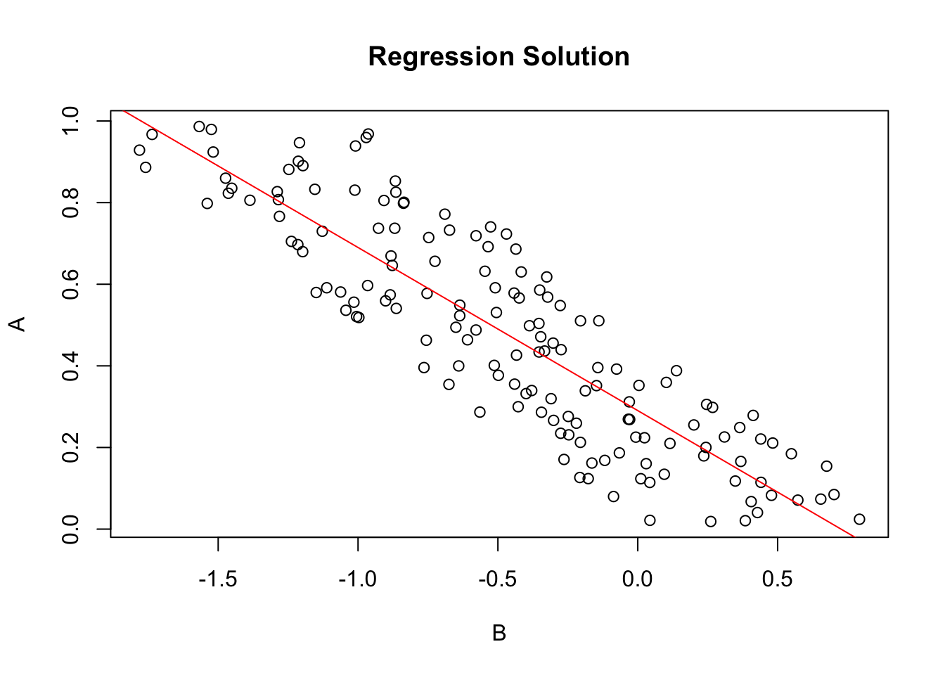

if(par3 == FALSE) abline(0.0, coef(lmxdf), col='red')
qqPlot(resid(lmxdf), main='QQplot of Residuals of Fit')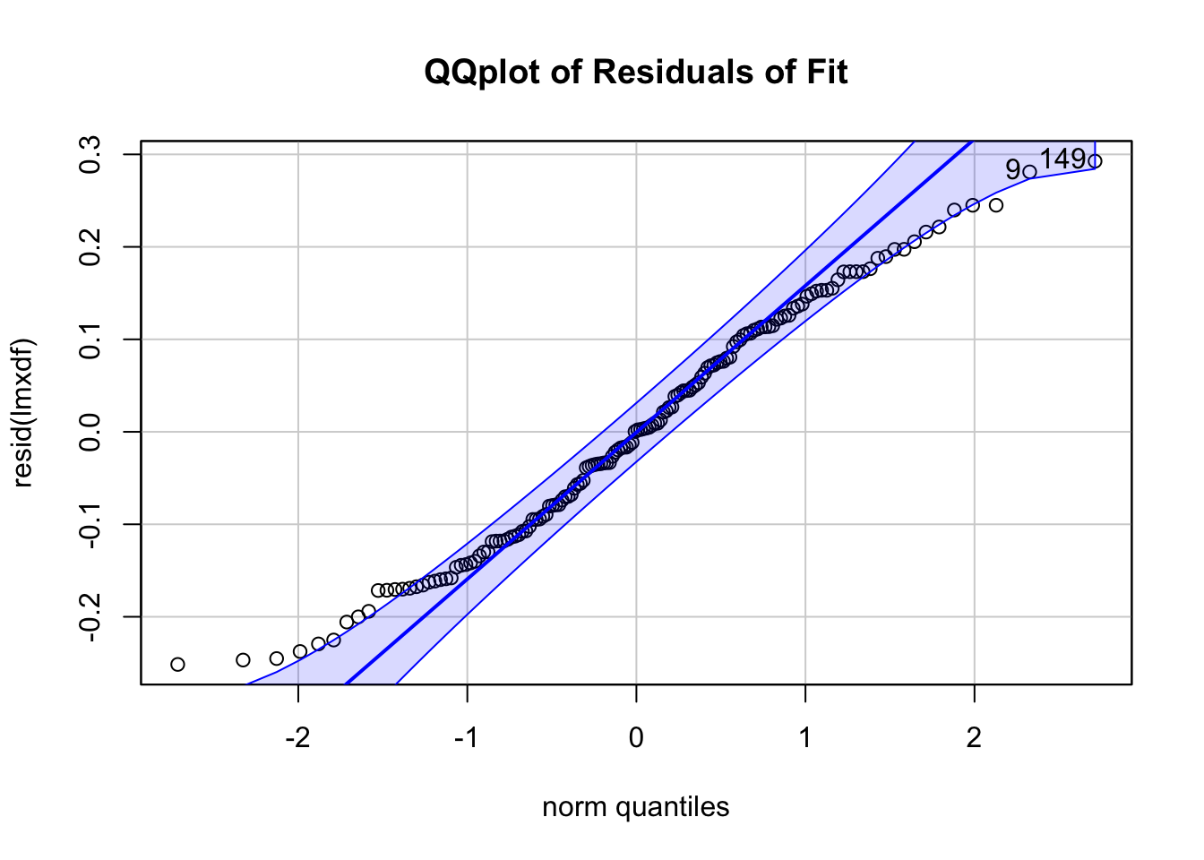

plot(xdf$X, resid(lmxdf), main='Scatterplot of Residuals of Model Fit')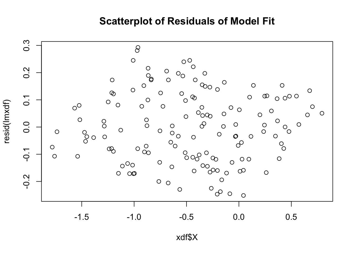

plot(lmxdf, which=4)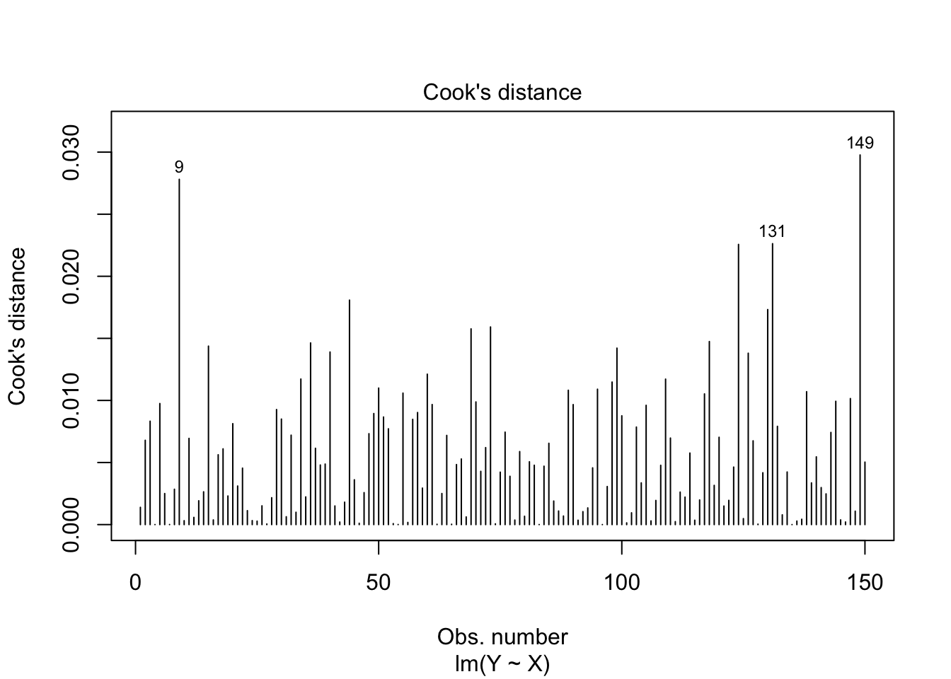

Selected columns
[1] "A"
[1] "B"


Result of Simple Linear Regression computation

Call:
lm(formula = Y ~ X, data = xdf)

Residuals:
      Min        1Q    Median        3Q       Max 
-0.251522 -0.107559  0.001211  0.106425  0.292664 

Coefficients:
            Estimate Std. Error t value Pr(>|t|)    
(Intercept)  0.29044    0.01349   21.53   <2e-16 ***
X           -0.39972    0.01793  -22.30   <2e-16 ***
---
Signif. codes:  0 '***' 0.001 '**' 0.01 '*' 0.05 '.' 0.1 ' ' 1

Residual standard error: 0.1294 on 148 degrees of freedom
Multiple R-squared:  0.7706,    Adjusted R-squared:  0.7691 
F-statistic: 497.2 on 1 and 148 DF,  p-value: < 2.2e-16


Fitting an Analysis of Variance Model
Call:
   aov(formula = lmxdf)

Terms:
                       X Residuals
Sum of Squares  8.322257  2.477201
Deg. of Freedom        1       148

Residual standard error: 0.1293748
Estimated effects may be unbalanced



Analysis of Variance Table

Response: Y
           Df Sum Sq Mean Sq F value    Pr(>F)    
X           1 8.3223  8.3223  497.21 < 2.2e-16 ***
Residuals 148 2.4772  0.0167                      
---
Signif. codes:  0 '***' 0.001 '**' 0.01 '*' 0.05 '.' 0.1 ' ' 1


95% Confidence Interval of R-squared
[1] "[0.721,0.814]"
[1] 149   9

To compute a Simple Linear Regression model, the R code uses the lm and summary functions which are part of the base R installation. A few more advanced elements were added to make the script more interesting:

• while the R-squared value (Section 71.3) is available through the lm and summary functions, the confidence interval has also been computed through the addition of “bootstrapping” (a form of simulation) based on the boot library and a custom-made function called rsq
• a Normal QQ Plot was added based on the car package
• two scatterplots and the Cook’s distance plot were also included (Cook’s distance is beyond the scope of this book)

74.5 Purpose

The Simple Linear Regression model is useful when the endogenous variable \(y\) can be adequately described/predicted by just one exogenous variable \(x\). A case study which illustrates the use of this model is provided later (Do Course Evaluations Make Sense?).

74.6 Pros & Cons

74.6.1 Pros

The Simple Linear Regression model has the following advantages:

• It can be computed with many software packages (even with spreadsheets).
• The interpretation is straightforward and many readers are familiar with this model.
• It can be easily illustrated with graphical representations.

74.6.2 Cons

The Simple Linear Regression model has the following disadvantages:

• It assumes that there is only one exogenous variable which is needed to adequately predict the endogenous variable.
• The model is sensitive to outliers.
• The model does not necessarily allow researchers to infer causation.

74.7 Simulation

The following R module simulates a Simple Linear Regression and shows how the prediction errors violate the underlying assumptions:

• https://compute.wessa.net/rwasp_regr.wasp

To compute the simulation on your local machine, the following script can be used in the R console:

set.seed(42)
x=0:10
y=x+2+1.5*rnorm(length(x))
print(x)
print(y)
plot(x,y,xlab='predictor,x',ylab='predicted y',main='Predictive Model',pch=16,cex=1.5,xlim=c(min(x)-.2*sd(x),max(x)+.2*sd(x)),ylim=c(min(y),max(y)+.2*sd(y)))
lmout=lm(y~x)
lines(x,lmout$fitted,col='red',lwd=2)
x0=mean(x)+sd(x)
y0=lmout$coefficients[[1]]+lmout$coefficients[[2]]*x0
x1=mean(x)-.5*sd(x)
y1=lmout$coefficients[[1]]+lmout$coefficients[[2]]*x1
arrows(x0,min(y)-.2*sd(y),x0,y0,col='blue',code=2)
arrows(x0,y0,min(x)-.2*sd(x),y0,col='blue',code=2)
arrows(x1,min(y)-.2*sd(y),x1,y1,col='blue',code=2)
arrows(x1,y1,min(x)-.2*sd(x),y1,col='blue',code=2)
for (i in 1:length(x))
{
  lines(c(x[i],x[i]),c(y[i],lmout$fitted[i]),col='darkgreen',lwd=1.5)
}
#legend(max(x)-3,mean(y)-.01*sd(x),c('regression line: red','predictions: blue','prediction errors: green'))
legend("bottomright",c('regression line-red','predictions-blue','prediction errors-green'))
#legend(max(x)-3,mean(y)-0.5*sd(x),'predictions-blue')
#legend(max(x)-3,mean(y)-1.0*sd(x),'prediction errors-green')
text(mean(x)-sd(x),max(y)+.15*sd(y),'Regression Line Minimizes',col='purple')
text(mean(x)-sd(x),max(y)-.10*sd(y),'Root-Mean-Square',col='purple')
text(mean(x)+0.4*sd(x),max(y)-.10*sd(y),'Prediction Error',col='darkgreen')

plot(x,lmout$residuals,xlab='predictor,x',ylab='prediction error (residual)',main='Residuals from Regression Fit',xlim=c(min(x)-.2*sd(x),max(x)+.2*sd(x)),pch=16,cex=1.5)
lines(c(min(x),max(x)),c(0,0),lwd=2)
for (i in 1:length(x))
{
  lines(c(x[i],x[i]),c(lmout$residuals[i],0),col='darkgreen',lwd=1.5)
}

z=x+5*(x/sd(x))^2+5*rnorm(length(x))
lmout2=lm(z~x)
plot(x,z,pch=16,cex=1.5,main='New data set - linear? (Not!)')
lines(x,lmout2$fitted,lwd=2,col='red')

plot(x,lmout2$residuals,pch=16,cex=1.5,main='Residual plot for new data',ylab='residual')
lines(c(min(x),max(x)),c(0,0),lwd=2)
fit=loess(lmout2$residuals~x,span=1,degree=2)
lines(fit$x,fit$fitted,col='red')

 [1]  0  1  2  3  4  5  6  7  8  9 10
 [1]  4.056438  2.152953  4.544693  5.949294  6.606402  6.840813 10.267283
 [8]  8.858011 13.027636 10.905929 13.957304

To compute the Simulation of the Simple Linear Regression model, the R code uses simulated data with the rnorm function and specifies the model \(y_i = \beta_0 + \beta_1 x_i + \epsilon_i\) where \(\beta_0 = 2\) and \(\beta_1 = 1\).

74.8 Example

The following analysis shows the Linear Regression Model for the relationship between Price and Horsepower.

Interactive Shiny app (click to load).

Open in new tab

The regression equation is \(Price = -1.3988 + 0.1454 Horsepower\) which implies that a car with \(Horsepower = 143.8\) will cost (on average) \(-1.3988 + 0.1454 * 143.8 \simeq 19.5\).

Legendre, Adrien-Marie. 1805. “Nouvelles méthodes Pour La détermination Des Orbites Des Comètes.”