The Box-Cox Normality Plot is closely related to the PPCC Plot. It uses the same iterative procedure but with a different objective: instead of identifying which distribution best fits the data, the Box-Cox Normality Plot finds the optimal power transformation parameter \(\lambda\) (based on the Box-Cox transformation (Box and Cox 1964)) that makes the data as close to normally distributed as possible.
The procedure works as follows:
a value for the transformation parameter \(\lambda\) is set to an initial value
all observations are transformed using the Box-Cox transformation for the current value of \(\lambda\)
the Normal Probability Plot (i.e. QQ Plot against the Normal Distribution) is computed for the transformed data
the Pearson Correlation Coefficient (of the Normal Probability Plot) is computed and stored together with the current value of \(\lambda\)
steps 2 through 4 are repeated until a (pre-specified) final value is reached for the transformation parameter
a plot is generated which shows all Pearson Correlation Coefficients against their respective \(\lambda\) values
The \(\lambda\) value that produces the highest correlation indicates the power transformation that brings the data closest to normality.
79.1.1 Full (Sign-Preserving) Power Transformation
The following sign-preserving, Box-Cox-like transformation is defined as
which is the default setting for the Box-Cox Normality Plot in this module. It is not the standard Box-Cox transformation: standard Box-Cox requires strictly positive data (or an additive shift), while the use of \(\text{sign}(Y)\) and \(|Y|\) allows this variant to handle negative values (except \(Y=0\) when \(\lambda=0\)).
Maximum correlation: 0.9990619
Optimal lambda: -0.01
bcPower Transformation to Normality
  Est Power Rounded Pwr Wald Lwr Bnd Wald Upr Bnd
x   -0.0146           0      -0.0892       0.0601

Likelihood ratio test that transformation parameter is equal to 0
 (log transformation)
                            LRT df    pval
LR test, lambda = (0) 0.1462913  1 0.70211

Likelihood ratio test that no transformation is needed
                          LRT df       pval
LR test, lambda = (1) 677.965  1 < 2.22e-16
[1]  75 157
[1]  75 413
To compute the Box-Cox Normality Plot, the R code iterates over values of \(\lambda\) between \(-2\) and \(2\) with a step size of \(0.01\). For each value of \(\lambda\), the data is transformed and the Pearson Correlation Coefficient between the Normal Quantiles (computed via qnorm(ppoints(x))) and the sorted transformed data is computed. The value of \(\lambda\) that produces the highest correlation is the optimal transformation parameter.
In addition to the graphical (correlation-based) approach, the powerTransform function from the car package computes a Maximum Likelihood Estimate (MLE) of \(\lambda\) for a parametric power-transformation model. In this example the data are positive, so the standard Box-Cox MLE is applicable; in general, standard Box-Cox requires strictly positive data (or a prior shift). The MLE approach provides a confidence interval and a formal hypothesis test for whether \(\lambda\) is significantly different from common values such as \(0\) (log transform) or \(1\) (no transform).
79.5 Purpose
The Box-Cox Normality Plot serves two main purposes:
It provides a visual and quantitative method to determine which power transformation brings the data closest to a Normal Distribution. This is particularly useful when normality is an assumption of subsequent analysis (e.g. hypothesis testing, linear regression).
It provides an estimate for \(\lambda\) which can be used to transform the data before further analysis. Note that the value of \(\lambda\) is typically rounded to a convenient value (see Table 79.1) if the rounded value falls within the confidence interval of the MLE estimate.
Note: the Box-Cox Normality Plot is also used in time series analysis to induce stationarity of the variance – see Chapter 150 for a detailed discussion.
79.6 Pros & Cons
79.6.1 Pros
The Box-Cox Normality Plot has the following advantages:
it provides a clear visual indication of the optimal transformation parameter
it is easy to interpret: a sharp peak in the plot indicates a well-defined optimal \(\lambda\)
it combines well with the QQ Plot to show the improvement in normality before and after transformation
the MLE approach provides a formal hypothesis test and confidence interval for \(\lambda\)
79.6.2 Cons
The Box-Cox Normality Plot has the following disadvantages:
the Box-Cox transformation mainly addresses skewness; it may reduce tail weight caused by right-skewness, but it typically cannot fix multimodality or intrinsically heavy-tailed symmetric distributions
the simple transformation requires strictly positive data; a constant may need to be added before the analysis is performed
there is no guarantee that any power transformation will achieve normality for a given dataset
79.7 Example
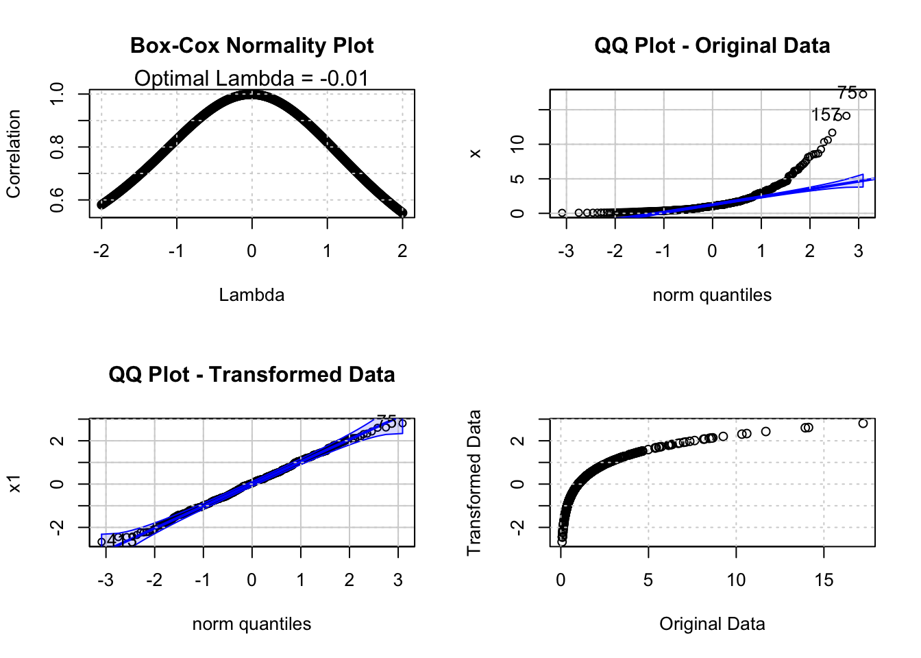
The following analysis shows the Box-Cox Normality Plot for the monthly marriages time series in Belgium. From the Tukey-Lambda PPCC Plot we already know that the distribution of this time series resembles a Uniform Distribution (see Section 78.8). The Box-Cox Normality Plot shows the optimal value of \(\lambda\) to transform the data towards normality.
The Box-Cox Normality Plot shows that the optimal \(\lambda\) is close to \(0\) (\(\ln Y\)) for the marriages time series. The QQ Plots confirm that the log-transformed data is closer to the Normal Distribution than the original data. The MLE output from powerTransform provides the exact estimate of \(\lambda\) and its confidence interval, which allows us to determine whether rounding to a convenient value (e.g. \(0\)) is appropriate.
79.8 Task
Compute the Box-Cox Normality Plot for the monthly divorces time series and interpret the results. Compare the optimal \(\lambda\) with the result of the PPCC Plot in Section 78.8. What does this tell you about the relationship between the two methods?
Box, George E. P., and David R. Cox. 1964. “An Analysis of Transformations.”Journal of the Royal Statistical Society. Series B (Methodological) 26 (2): 211–52. https://doi.org/10.1111/j.2517-6161.1964.tb00553.x.