50  Maxwell-Boltzmann Distribution

The Maxwell-Boltzmann distribution describes the speed of particles in an ideal gas at thermal equilibrium. It is one of the cornerstones of statistical mechanics and kinetic theory, connecting the macroscopic quantity temperature to the microscopic distribution of molecular speeds.

Formally, the random variate \(V\) defined for the range \(V \geq 0\), is said to have a Maxwell-Boltzmann Distribution (i.e. \(V \sim \text{Maxwell}(a)\)) with scale parameter \(a > 0\). In the physical context, \(a = \sqrt{k_BT/m}\) where \(k_B\) is the Boltzmann constant, \(T\) is the absolute temperature, and \(m\) is the molecular mass. The Maxwell-Boltzmann distribution is a scaled Chi distribution with \(k = 3\) degrees of freedom: if \(X \sim \chi(3)\) then \(aX \sim \text{Maxwell}(a)\).

50.1 Probability Density Function

\[ f(v) = \sqrt{\frac{2}{\pi}}\,\frac{v^2}{a^3}\,\exp\!\left(-\frac{v^2}{2a^2}\right), \quad v \geq 0 \]

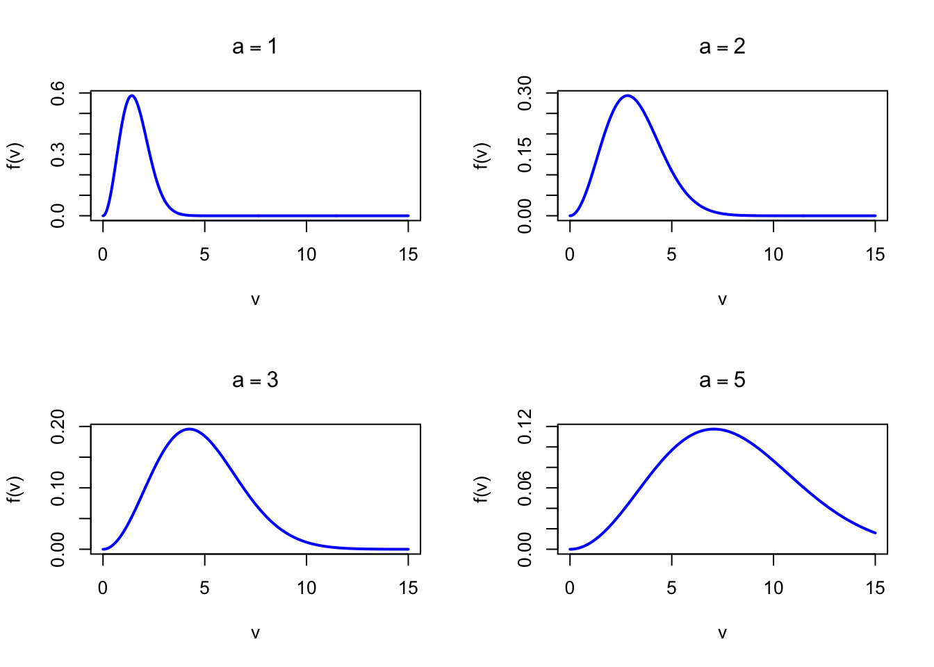
The figure below shows examples of the Maxwell-Boltzmann Probability Density Function for different scale values.

dmaxwell <- function(v, a) {
  ifelse(v >= 0, sqrt(2/pi) * v^2 / a^3 * exp(-v^2 / (2 * a^2)), 0)
}

par(mfrow = c(2, 2))
v <- seq(0, 15, length = 500)

plot(v, dmaxwell(v, 1), type = "l", lwd = 2, col = "blue",
     xlab = "v", ylab = "f(v)", main = expression(a == 1))

plot(v, dmaxwell(v, 2), type = "l", lwd = 2, col = "blue",
     xlab = "v", ylab = "f(v)", main = expression(a == 2))

plot(v, dmaxwell(v, 3), type = "l", lwd = 2, col = "blue",
     xlab = "v", ylab = "f(v)", main = expression(a == 3))

plot(v, dmaxwell(v, 5), type = "l", lwd = 2, col = "blue",
     xlab = "v", ylab = "f(v)", main = expression(a == 5))

par(mfrow = c(1, 1))

Figure 50.1: Maxwell-Boltzmann Probability Density Function for various scale values

50.2 Purpose

The Maxwell-Boltzmann distribution is the fundamental speed distribution for particles in thermal equilibrium. It connects microscopic particle dynamics to macroscopic thermodynamic properties and underpins much of statistical physics. Common applications include:

• Kinetic theory of gases: distribution of molecular speeds at a given temperature
• Molecular dynamics simulations: initialization and validation of velocity distributions
• Diffusion modeling: relating diffusion coefficients to particle speed distributions
• Stellar atmospheres: spectral line broadening from thermal Doppler shifts
• Thermodynamic equilibrium: deriving transport properties (viscosity, thermal conductivity)

Relation to the Chi distribution. The Maxwell-Boltzmann distribution is the Chi distribution with \(k = 3\) degrees of freedom, scaled by \(a\). This arises because the speed \(v = \sqrt{v_x^2 + v_y^2 + v_z^2}\) is the Euclidean norm of three independent \(N(0, a^2)\) velocity components.

50.3 Distribution Function

\[ F(v) = \text{erf}\!\left(\frac{v}{a\sqrt{2}}\right) - \sqrt{\frac{2}{\pi}}\,\frac{v}{a}\,\exp\!\left(-\frac{v^2}{2a^2}\right), \quad v \geq 0 \]

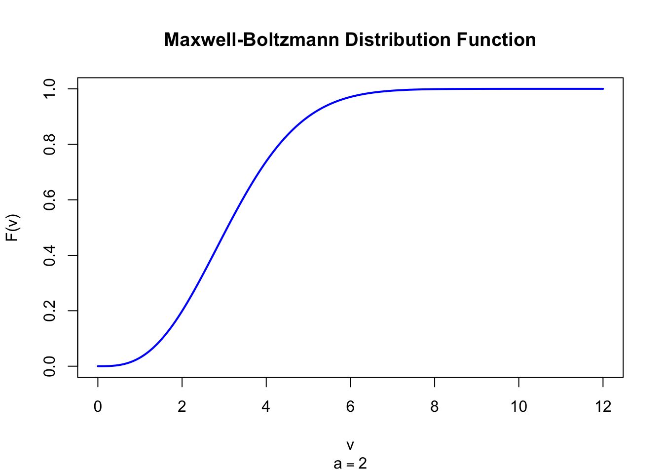
where \(\text{erf}(z) = \frac{2}{\sqrt{\pi}}\int_0^z e^{-t^2}\,dt\). In R, the CDF can be computed via the Chi-squared distribution: pchisq((v/a)^2, df = 3).

The figure below shows the Maxwell-Boltzmann Distribution Function for \(a = 2\).

pmaxwell <- function(v, a) {
  ifelse(v >= 0, pchisq((v/a)^2, df = 3), 0)
}

v <- seq(0, 12, length = 500)
plot(v, pmaxwell(v, 2), type = "l", lwd = 2, col = "blue",
     xlab = "v", ylab = "F(v)", main = "Maxwell-Boltzmann Distribution Function",
     sub = expression(a == 2))

Figure 50.2: Maxwell-Boltzmann Distribution Function (a = 2)

50.4 Moment Generating Function

The moment generating function has no simple closed form. Raw moments are computed directly from the density:

\[ \mu_n' = a^n\, 2^{n/2}\,\frac{\Gamma\!\left(\frac{n+3}{2}\right)}{\Gamma\!\left(\frac{3}{2}\right)} \]

50.5 Expected Value

\[ \text{E}(V) = 2a\sqrt{\frac{2}{\pi}} \]

This is the mean speed \(\bar{v}\) of the particles. In the physical context with \(a = \sqrt{k_BT/m}\):

\[ \bar{v} = \sqrt{\frac{8k_BT}{\pi m}} \]

50.6 Variance

\[ \text{V}(V) = a^2\left(3 - \frac{8}{\pi}\right) \]

50.7 Median

The median has no simple closed form and must be computed numerically:

# Median of Maxwell-Boltzmann(a): numerical
a <- 2
pmaxwell <- function(v, a) pchisq((v/a)^2, df = 3)
uniroot(function(v) pmaxwell(v, a) - 0.5, c(0.001, 100))$root

[1] 3.076345

50.8 Mode

\[ \text{Mo}(V) = a\sqrt{2} \]

The mode is the most probable speed \(v_p\). In the physical context:

\[ v_p = \sqrt{\frac{2k_BT}{m}} \]

50.9 Coefficient of Skewness

\[ g_1 = \frac{2\sqrt{2}\,(16 - 5\pi)}{(3\pi - 8)^{3/2}} \approx 0.4857 \]

This is a fixed constant, independent of \(a\). The Maxwell-Boltzmann distribution is always positively skewed (right-skewed).

50.10 Coefficient of Kurtosis

\[ g_2 = 3 + \frac{4\left(-96 + 40\pi - 3\pi^2\right)}{(3\pi - 8)^2} \approx 3.108 \]

The excess kurtosis \(g_2 - 3 \approx 0.108\) is small and positive, indicating slightly heavier tails than the Normal distribution. This is a fixed constant, independent of \(a\).

50.11 Parameter Estimation

The MLE of \(a^2\) is:

\[ \hat a^2 = \frac{1}{3n}\sum_{i=1}^n v_i^2 \]

This follows from the equivalence with the Chi distribution: \(V^2/a^2 \sim \chi^2(3)\), so the sufficient statistic is \(\sum v_i^2\).

set.seed(42)
a_true <- 2

# Simulate Maxwell-Boltzmann data via 3D Gaussian speed
vx <- rnorm(200, 0, a_true)
vy <- rnorm(200, 0, a_true)
vz <- rnorm(200, 0, a_true)
v_obs <- sqrt(vx^2 + vy^2 + vz^2)

# MLE
a_hat <- sqrt(mean(v_obs^2) / 3)
cat("MLE a:", round(a_hat, 4), "\n")
cat("True a:", a_true, "\n")

MLE a: 1.9732 
True a: 2 

50.12 R Module

50.12.1 RFC

The Maxwell-Boltzmann Distribution module is available in RFC under the menu “Distributions / Maxwell-Boltzmann Distribution”.

50.12.2 Direct app link

• https://shiny.wessa.net/maxwellboltzmann/

50.12.3 R Code

The following code demonstrates Maxwell-Boltzmann probability calculations:

a <- 2

# Custom density function
dmaxwell <- function(v, a) {
  ifelse(v >= 0, sqrt(2/pi) * v^2 / a^3 * exp(-v^2 / (2 * a^2)), 0)
}

# Custom CDF using Chi-squared
pmaxwell <- function(v, a) {
  ifelse(v >= 0, pchisq((v/a)^2, df = 3), 0)
}

# Density at v = 3
dmaxwell(3, a)

# P(V <= 3): distribution function
pmaxwell(3, a)

# Characteristic speeds
cat("Most probable speed (mode):", a * sqrt(2), "\n")
cat("Mean speed:", 2 * a * sqrt(2/pi), "\n")
cat("RMS speed:", a * sqrt(3), "\n")

[1] 0.2914146
[1] 0.4778328
Most probable speed (mode): 2.828427 
Mean speed: 3.191538 
RMS speed: 3.464102 

50.13 Example

Consider nitrogen (\(\text{N}_2\), molar mass \(M = 0.028\) kg/mol) molecules at room temperature \(T = 300\) K. Using \(k_B = 1.380649 \times 10^{-23}\) J/K and \(N_A = 6.02214 \times 10^{23}\) mol\(^{-1}\), the molecular mass is \(m = M/N_A\) and the scale parameter is \(a = \sqrt{k_BT/m}\).

# Physical constants
kB <- 1.380649e-23   # Boltzmann constant (J/K)
NA_const <- 6.02214076e23  # Avogadro's number (1/mol)

# Nitrogen at 300 K
M <- 0.028           # Molar mass (kg/mol)
T_kelvin <- 300      # Temperature (K)
m <- M / NA_const    # Molecular mass (kg)

# Scale parameter
a <- sqrt(kB * T_kelvin / m)

# Characteristic speeds (m/s)
v_p   <- a * sqrt(2)
v_avg <- 2 * a * sqrt(2/pi)
v_rms <- a * sqrt(3)

cat("Scale parameter a:", round(a, 2), "m/s\n")
cat("Most probable speed v_p:", round(v_p, 2), "m/s\n")
cat("Mean speed v_avg:", round(v_avg, 2), "m/s\n")
cat("RMS speed v_rms:", round(v_rms, 2), "m/s\n")

# P(V > 600 m/s) — fraction of fast molecules
pmaxwell <- function(v, a) pchisq((v/a)^2, df = 3)
cat("P(V > 600 m/s):", round(1 - pmaxwell(600, a), 4), "\n")

Scale parameter a: 298.47 m/s
Most probable speed v_p: 422.1 m/s
Mean speed v_avg: 476.29 m/s
RMS speed v_rms: 516.96 m/s
P(V > 600 m/s): 0.2571 

Interactive Shiny app (click to load).

Open in new tab

50.14 Random Number Generator

Maxwell-Boltzmann random variates are generated from three independent Normal variates. Since the speed is the Euclidean norm of the 3D velocity vector:

\[ V = \sqrt{V_x^2 + V_y^2 + V_z^2} \sim \text{Maxwell}(a) \quad \text{when } V_x, V_y, V_z \overset{\text{i.i.d.}}{\sim} N(0, a^2) \]

set.seed(123)
n <- 1000; a <- 2

# Generate Maxwell-Boltzmann via 3D Gaussian magnitude
vx <- rnorm(n, 0, a)
vy <- rnorm(n, 0, a)
vz <- rnorm(n, 0, a)
v_sim <- sqrt(vx^2 + vy^2 + vz^2)

cat("Simulated mean:", round(mean(v_sim), 4), "\n")
cat("Theoretical mean:", 2 * a * sqrt(2/pi), "\n")
cat("Simulated var:", round(var(v_sim), 4), "\n")
cat("Theoretical var:", a^2 * (3 - 8/pi), "\n")

Simulated mean: 3.1705 
Theoretical mean: 3.191538 
Simulated var: 1.7881 
Theoretical var: 1.814084 

Interactive Shiny app (click to load).

Open in new tab

50.15 Property 1: 3D Gaussian Speed

If \(V_x, V_y, V_z \overset{\text{i.i.d.}}{\sim} N(0, a^2)\) then:

\[ V = \sqrt{V_x^2 + V_y^2 + V_z^2} \sim \text{Maxwell}(a) \]

This makes the Maxwell-Boltzmann distribution the natural model for the speed (magnitude of the velocity vector) of particles whose velocity components are independently and identically normally distributed.

50.16 Property 2: Three Characteristic Speeds

The Maxwell-Boltzmann distribution has three characteristic speeds that appear frequently in kinetic theory:

\[ v_p = a\sqrt{2} < \bar{v} = 2a\sqrt{\frac{2}{\pi}} < v_{\text{rms}} = a\sqrt{3} \]

The most probable speed \(v_p\) (mode) is always less than the mean speed \(\bar{v}\), which is always less than the root-mean-square speed \(v_{\text{rms}}\). Their ratios are universal constants independent of temperature or molecular mass:

\[ v_p : \bar{v} : v_{\text{rms}} = 1 : 1.128 : 1.225 \]

50.17 Property 3: Energy Distribution

If \(V \sim \text{Maxwell}(a)\) then the kinetic energy \(E = \frac{1}{2}mv^2\) follows a Gamma distribution:

\[ E \sim \text{Gamma}\!\left(\frac{3}{2},\, \frac{1}{k_BT}\right) \]

The mean kinetic energy is \(\text{E}(E) = \frac{3}{2}k_BT\), which is the equipartition theorem result. See Chapter 29.

50.18 Property 4: Constant Shape Statistics

The coefficient of variation, skewness, and kurtosis of the Maxwell-Boltzmann distribution are all universal constants, independent of the scale parameter \(a\) (and therefore independent of temperature and molecular mass):

\[ \text{CV} = \sqrt{\frac{3\pi - 8}{8}} \approx 0.422 \]

50.19 Related Distributions 1: Chi Distribution

The Maxwell-Boltzmann distribution is the Chi distribution with \(k = 3\) degrees of freedom, scaled by \(a\): \(\text{Maxwell}(a) = a \cdot \chi(3)\) (see Chapter 22).

50.20 Related Distributions 2: Rayleigh Distribution

The Rayleigh distribution is the 2D analogue of the Maxwell-Boltzmann distribution — it describes the magnitude of a 2D Gaussian vector, whereas the Maxwell-Boltzmann describes the magnitude of a 3D Gaussian vector: \(\text{Rayleigh}(\sigma) = \sigma \cdot \chi(2)\) while \(\text{Maxwell}(a) = a \cdot \chi(3)\) (see Chapter 34).

50.21 Related Distributions 3: Normal Distribution

The individual velocity components \(V_x, V_y, V_z\) each follow a Normal distribution \(N(0, a^2)\), and the Maxwell-Boltzmann distribution arises as the norm of the 3D velocity vector (see Chapter 20).

50.22 Related Distributions 4: Gamma Distribution

The kinetic energy \(E = \frac{1}{2}mv^2\) of a Maxwell-Boltzmann distributed particle follows a Gamma distribution with shape \(3/2\) and rate \(1/(k_BT)\) (see Chapter 29).