The Lognormal distribution is the natural model for positive-valued quantities that arise through multiplicative growth or accumulation. Where the Normal distribution describes phenomena built up by addition, the Lognormal describes phenomena built up by multiplication — income, stock prices, environmental concentrations, and biological sizes all tend to follow it.
Formally, the random variate \(X\) defined for the range \(X > 0\), is said to have a Lognormal Distribution (i.e. \(X \sim \text{LnN}(\mu, \sigma^2)\)) if \(\ln(X)\) follows a Normal Distribution with mean \(\mu \in \mathbb{R}\) and variance \(\sigma^2 > 0\).
Parameterization note. The parameters \(\mu\) and \(\sigma\) are the mean and standard deviation of \(\ln(X)\), not of \(X\) itself. The mean and variance of \(X\) are more complex functions of \(\mu\) and \(\sigma\) (see the Expected Value and Variance sections below). In R, these parameters are named meanlog (\(= \mu\)) and sdlog (\(= \sigma\)). For large values of \(\sigma\), the density peak concentrates very close to zero and the distribution becomes heavily right-skewed.
28.1 Probability Density Function
\[
f(x) = \frac{1}{x \sigma \sqrt{2\pi}} \exp\!\left(-\frac{(\ln x - \mu)^2}{2\sigma^2}\right), \quad x > 0
\]
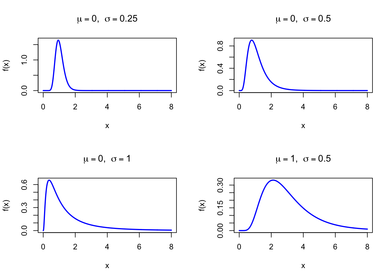
The figure below shows examples of the Lognormal Probability Density Function for different parameter combinations.
Code
par(mfrow =c(2, 2))x <-seq(0.001, 8, length =1000)plot(x, dlnorm(x, meanlog =0, sdlog =0.25), type ="l", lwd =2, col ="blue",xlab ="x", ylab ="f(x)", main =expression(paste(mu ==0, ", ", sigma ==0.25)))plot(x, dlnorm(x, meanlog =0, sdlog =0.5), type ="l", lwd =2, col ="blue",xlab ="x", ylab ="f(x)", main =expression(paste(mu ==0, ", ", sigma ==0.5)))plot(x, dlnorm(x, meanlog =0, sdlog =1), type ="l", lwd =2, col ="blue",xlab ="x", ylab ="f(x)", main =expression(paste(mu ==0, ", ", sigma ==1)))plot(x, dlnorm(x, meanlog =1, sdlog =0.5), type ="l", lwd =2, col ="blue",xlab ="x", ylab ="f(x)", main =expression(paste(mu ==1, ", ", sigma ==0.5)))par(mfrow =c(1, 1))
Figure 28.1: Lognormal Probability Density Function for various parameter combinations
28.2 Purpose
The Lognormal distribution models positive quantities that arise as the product of many small independent factors. By the multiplicative analogue of the Central Limit Theorem, the logarithm of such a product is approximately Normal, so the product itself is approximately Lognormal. Common applications include:
Household income and individual wealth distributions
Stock prices and financial asset returns (multiplicative period-by-period changes)
Environmental concentrations: pollutant levels, water quality measurements
Biological sizes, growth rates, and incubation times
Latency and response times in computing and telecommunications systems
Relation to the discrete setting. There is no standard discrete counterpart of the Lognormal distribution. Its defining feature — the logarithm of the variable is Normal — has no natural discrete analog. The closest conceptual relatives are the Geometric and Negative Binomial distributions, which arise from multiplicative processes in discrete state spaces, and the Logarithmic series distribution, which has a log-linear tail. The Lognormal stands apart from the other continuous distributions in this chapter because it arises from multiplicative rather than additive accumulation of independent effects.
28.3 Distribution Function
\[
F(x) = \Phi\!\left(\frac{\ln x - \mu}{\sigma}\right), \quad x > 0
\]
where \(\Phi(\cdot)\) denotes the standard Normal distribution function (see Chapter 20).
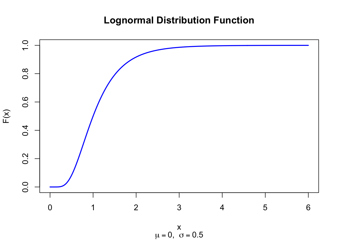
The figure below shows the Lognormal Distribution Function for \(\mu = 0\) and \(\sigma = 0.5\).
Code
x <-seq(0, 6, length =500)plot(x, plnorm(x, meanlog =0, sdlog =0.5), type ="l", lwd =2, col ="blue",xlab ="x", ylab ="F(x)", main ="Lognormal Distribution Function",sub =expression(paste(mu ==0, ", ", sigma ==0.5)))
Figure 28.2: Lognormal Distribution Function (mu = 0, sigma = 0.5)
28.4 Moment Generating Function
The moment generating function \(M_X(t) = \text{E}(e^{tX})\) does not exist for any \(t > 0\). Because \(\text{E}(X^n) = \exp(n\mu + n^2\sigma^2/2)\) grows super-exponentially in \(n\), the Taylor series \(\sum_{n=0}^{\infty} t^n \text{E}(X^n)/n!\) diverges for all \(t > 0\). All moments of the Lognormal distribution are nevertheless finite.
28.5 1st Uncentered Moment
\[
\mu_1' = e^{\mu + \sigma^2/2}
\]
28.6 2nd Uncentered Moment
\[
\mu_2' = e^{2\mu + 2\sigma^2}
\]
28.7 3rd Uncentered Moment
\[
\mu_3' = e^{3\mu + 9\sigma^2/2}
\]
28.8 4th Uncentered Moment
\[
\mu_4' = e^{4\mu + 8\sigma^2}
\]
The general formula is \(\mu_n' = \text{E}(X^n) = \exp(n\mu + n^2\sigma^2/2)\).
The Lognormal distribution is always positively skewed. As \(\sigma \to 0\), the skewness approaches 0 (the distribution becomes approximately symmetric around \(e^\mu\)).
The Lognormal distribution always has Pearson kurtosis greater than 3 (\(g_2 > 3\) for all \(\sigma > 0\)), indicating heavier tails than the Normal distribution.
28.18 Parameter Estimation
Taking logarithms transforms the problem to Normal parameter estimation. The maximum likelihood estimators are:
Annual household incomes in a region are modelled as Lognormal with \(\mu = 10\) (meanlog) and \(\sigma = 0.5\) (sdlog). The median income is \(e^{10} \approx 22{,}026\) EUR and the mean income is \(e^{10 + 0.25} \approx 28{,}403\) EUR. We compute several policy-relevant quantities:
mu_log <-10sd_log <-0.5# Median incomecat("Median income (EUR):", round(exp(mu_log)), "\n")# Mean incomecat("Mean income (EUR):", round(exp(mu_log + sd_log^2/2)), "\n")# P(income < 15000): share of households below a thresholdcat("P(income < 15000):", round(plnorm(15000, meanlog = mu_log, sdlog = sd_log), 4), "\n")# 90th percentile incomecat("90th percentile (EUR):", round(qlnorm(0.9, meanlog = mu_log, sdlog = sd_log)), "\n")
Median income (EUR): 22026
Mean income (EUR): 24959
P(income < 15000): 0.2211
90th percentile (EUR): 41805
By definition, if \(Z \sim \text{N}(\mu, \sigma^2)\) then \(X = e^Z \sim \text{LnN}(\mu, \sigma^2)\). Thus Lognormal random variates are generated by exponentiating Normal random variates:
28.22 Property 1: Defining Relationship with the Normal Distribution
The Lognormal distribution is defined by its relationship to the Normal distribution: if \(Y \sim \text{N}(\mu, \sigma^2)\) then \(X = e^Y \sim \text{LnN}(\mu, \sigma^2)\). Equivalently, \(\ln(X) \sim \text{N}(\mu, \sigma^2)\) (see Chapter 20).
28.23 Property 2: Closure Under Multiplication
If \(X_1 \sim \text{LnN}(\mu_1, \sigma_1^2)\) and \(X_2 \sim \text{LnN}(\mu_2, \sigma_2^2)\) are independent, then their product is also Lognormal:
This follows from the fact that \(\ln(X_1 X_2) = \ln X_1 + \ln X_2\) and the sum of independent Normals is Normal.
28.24 Property 3: Concentration as Shape Parameter Shrinks
As \(\sigma \to 0\), the Lognormal distribution degenerates: it concentrates all mass at \(e^\mu\). The mean, median, and mode all converge to \(e^\mu\), and the distribution becomes approximately Normal centered at \(e^\mu\).
28.25 Related Distributions 1: Defined via Normal
The Lognormal distribution is defined through the Normal distribution: \(\ln(X) \sim \text{N}(\mu, \sigma^2)\) implies \(X \sim \text{LnN}(\mu, \sigma^2)\) (see Chapter 20).
28.26 Related Distributions 2: Box-Cox Power Transform
The Box-Cox normality transform (see Chapter 79) generalizes the log transformation used to define the Lognormal. Finding the power parameter \(\lambda\) that most nearly normalizes a positive dataset subsumes the log transformation (\(\lambda = 0\) in the Box-Cox convention) as the special case corresponding to the Lognormal model.