%%{init: {'theme': 'base', 'securityLevel': 'loose', 'flowchart': {'htmlLabels': true}, 'themeVariables': { 'primaryColor': '#E3F2FD', 'primaryTextColor': '#1565C0', 'primaryBorderColor': '#1565C0', 'lineColor': '#666666', 'secondaryColor': '#E8F5E9', 'tertiaryColor': '#FFF3E0', 'fontSize': '14px'}}}%%
flowchart LR
    S1["<b>STEP 1: What is your PURPOSE?</b><br/><i>Choose your primary goal</i>"]
    S1 --> Describe["🔵 Describe / Explore"]
    S1 --> Test["🟢 Test hypothesis"]
    S1 --> Model["🟠 Build model / Predict"]

    Describe --> APath["→ <b>Path A</b><br/>Description & Exploration"]
    Test --> BPath["→ <b>Path B</b><br/>Hypothesis Testing"]
    Model --> MSplit["<b>STEP 2: Data STRUCTURE?</b><br/><i>Modeling</i>"]
    MSplit --> CPath["→ <b>Path C</b><br/>Modeling (Non-sequential)"]
    MSplit --> DPath["→ <b>Path D</b><br/>Modeling (Time Series)"]

    classDef stepBox fill:#F5F5F5,stroke:#424242,stroke-width:2px,color:#333
    classDef blueBox fill:#E3F2FD,stroke:#1565C0,stroke-width:2px,color:#1565C0
    classDef greenBox fill:#E8F5E9,stroke:#2E7D32,stroke-width:2px,color:#2E7D32
    classDef orangeBox fill:#FFF3E0,stroke:#EF6C00,stroke-width:2px,color:#EF6C00
    classDef purpleBox fill:#F3E5F5,stroke:#7B1FA2,stroke-width:2px,color:#7B1FA2
    classDef destBox fill:#fff,stroke:#333,stroke-width:2px,color:#333,font-weight:bold

    class S1 stepBox
    class Describe,APath blueBox
    class Test,BPath greenBox
    class Model,MSplit,CPath orangeBox
    class DPath purpleBox

    click APath "#sec-flowchart-path-a"
    click BPath "#sec-flowchart-path-b"
    click CPath "#sec-flowchart-path-c"
    click DPath "#sec-flowchart-path-d"
Appendix A — Method Selection Guide
This guide helps you choose the appropriate statistical method for your situation. Unlike typical “decision trees” that jump straight to data types and sample sizes, we start with the most important question: What are you trying to accomplish?
A.1 How to Use This Guide
Start with the Purpose Hub below, then follow the flowchart for your path. Click any destination box (marked with →) to jump directly to that section.
A.1.1 Quick-Reference Table
If you already know your research question, use this table to jump directly to the right method.
| Research Question | Method | Chapter | App |
|---|---|---|---|
| What does my data look like? | Descriptive statistics (mean, SD, quantiles) | 📖 | 🔗 |
| Are there measurement or data quality issues? | Data quality forensics | 📖 | 🔗 |
| Predict a single value (no covariates) | Mean / median / trimmed / geometric / harmonic / midrange | 📖 | 🔗 |
| Test/CI for central tendency (no model) | Bootstrap / Blocked bootstrap | 📖 | 🔗 |
| Is my data normally distributed? | QQ plot, Shapiro-Wilk, K-S test (with Lilliefors correction) | 📖 | 🔗 |
| Are there outliers? | Box plot, Z-scores | 📖 | 🔗 |
| Is the mean different from a value? | One-sample t-test | 📖 | 🔗 |
| Are two group means different? | Two-sample t-test / Welch’s | 📖 | 🔗 |
| Are paired measurements different? | Paired t-test | 📖 | 🔗 |
| Are two groups equivalent? | TOST equivalence test | 📖 | 🔗 |
| Are 3+ group means different? | ANOVA | 📖 | 🔗 |
| Are two categorical variables associated? | Chi-squared test | 📖 | 🔗 |
| Is there a linear relationship? | Correlation test (Pearson / Spearman) | 📖 | 🔗 |
| Does X predict Y (continuous)? | Linear regression | 📖 | 🔗 |
| Does X predict Y (binary)? | Logistic regression | 📖 | 🔗 |
| Classify cases into categories? | Logistic regression / ctree / Naive Bayes | 📖 | 🔗 |
| Forecast a time series? | ARIMA / Holt-Winters | 📖 | 🔗 |
| Does an external event affect a time series? | Intervention analysis | 📖 | 🔗 |
| Does X dynamically influence Y over time? | Transfer function / CCF | 📖 | 🔗 |
| Does data fit a specific distribution? | K-S test / Chi-squared GoF | 📖 | 🔗 |
A.1.2 Path A: Description & Exploration
%%{init: {'theme': 'base', 'securityLevel': 'loose', 'flowchart': {'htmlLabels': true}, 'themeVariables': { 'primaryColor': '#E3F2FD', 'primaryTextColor': '#1565C0', 'primaryBorderColor': '#1565C0', 'lineColor': '#666666', 'fontSize': '14px'}}}%%
flowchart LR
    AStart["<b>Describe or Explore?</b>"]
    AStart --> ADescribe["🔵 Describe"]
    AStart --> AExplore["🔵 Explore"]

    ADescribe --> A1["→ <b>A1</b><br/>Pure Description"]
    AExplore --> A2["→ <b>A2</b><br/>Exploratory Analysis"]

    classDef blueBox fill:#E3F2FD,stroke:#1565C0,stroke-width:2px,color:#1565C0
    classDef destBox fill:#fff,stroke:#333,stroke-width:2px,color:#333,font-weight:bold

    class AStart,ADescribe,AExplore blueBox
    class A1,A2 destBox

    click A1 "#a1-pure-description"
    click A2 "#a2-exploratory-data-analysis-eda"
NoteData Quality Forensics App
For a more comprehensive diagnostic workflow (beyond the examples in Path A), use the app: https://shiny.wessa.net/dataqualityforensics/.
A.1.3 Path B: Hypothesis Testing
%%{init: {'theme': 'base', 'securityLevel': 'loose', 'flowchart': {'htmlLabels': true}, 'themeVariables': { 'primaryColor': '#E8F5E9', 'primaryTextColor': '#2E7D32', 'primaryBorderColor': '#2E7D32', 'lineColor': '#666666', 'fontSize': '14px'}}}%%
flowchart LR
    BStart["<b>STEP 2: Data TYPE?</b><br/><i>Hypothesis testing</i>"]
    BStart --> BNum["🟢 Numeric"]
    BStart --> BCat["🟢 Categorical"]
    BStart --> BDist["🟢 Distribution fit"]

    BCat --> B5["→ <b>B5</b><br/>Association Tests"]
    BDist --> B6["→ <b>B6</b><br/>Goodness-of-Fit"]

    BNum --> BGroups["<b>STEP 3: How MANY groups?</b>"]
    BGroups --> B1["🟢 1 sample"]
    BGroups --> B2g["🟢 2 groups"]
    BGroups --> B3g["🟢 3+ groups"]

    B1 --> B2["→ <b>B2</b><br/>One-Sample Tests"]
    B2g --> B3["→ <b>B3</b><br/>Two-Sample Tests"]
    B3g --> B4["→ <b>B4</b><br/>Multi-Group Tests"]

    classDef greenBox fill:#E8F5E9,stroke:#2E7D32,stroke-width:2px,color:#2E7D32
    classDef destBox fill:#fff,stroke:#333,stroke-width:2px,color:#333,font-weight:bold

    class BStart,BNum,BCat,BDist,BGroups,B1,B2g,B3g greenBox
    class B2,B3,B4,B5,B6 destBox

    click B2 "#b2-one-sample-tests"
    click B3 "#b3-two-sample-tests"
    click B4 "#b4-more-than-two-groups"
    click B5 "#b5-association-and-correlation-tests"
    click B6 "#b6-goodness-of-fit-tests"
NoteCentral Tendency Without a Model
If your goal is to test or quantify a single central tendency (no predictors), use the Bootstrap Plot for CIs/tests of mean, median, or trimmed mean. For dependent or time‑ordered data, use the Blocked Bootstrap Plot. Apps: https://shiny.wessa.net/bootstrap/.
A.1.4 Path C: Modeling & Prediction
%%{init: {'theme': 'base', 'securityLevel': 'loose', 'flowchart': {'htmlLabels': true}, 'themeVariables': { 'primaryColor': '#FFF3E0', 'primaryTextColor': '#EF6C00', 'primaryBorderColor': '#EF6C00', 'lineColor': '#666666', 'fontSize': '14px'}}}%%
flowchart LR
    CStart["<b>STEP 2: Outcome TYPE?</b><br/><i>Modeling</i>"]
    CStart --> CCont["🟠 Continuous"]
    CStart --> CBin["🟠 Binary"]
    CStart --> CCount["🟠 Count"]
    CStart --> CAny["🟠 Any type"]

    CCont --> C2Reg["→ <b>C2</b><br/>Linear Regression"]
    CBin --> C2Log["→ <b>C2</b><br/>Logistic Regression"]
    CCount --> C2Pois["→ <b>C2</b><br/>Poisson/GLM"]
    CAny --> C2Tree["→ <b>C2</b><br/>ctree - flexible"]

    C2Reg --> C6["→ <b>C6</b><br/>Model Diagnostics"]
    C2Log --> C6
    C2Pois --> C6
    C2Tree --> C6

    classDef orangeBox fill:#FFF3E0,stroke:#EF6C00,stroke-width:2px,color:#EF6C00
    classDef destBox fill:#fff,stroke:#333,stroke-width:2px,color:#333,font-weight:bold

    class CStart,CCont,CBin,CCount,CAny orangeBox
    class C2Reg,C2Log,C2Pois,C2Tree,C6 destBox

    click C2Reg "#c2-choosing-a-regression-model"
    click C2Log "#c2-choosing-a-regression-model"
    click C2Pois "#c2-choosing-a-regression-model"
    click C2Tree "#c2-choosing-a-regression-model"
    click C6 "#sec-c6-model-diagnostics"
NoteBaseline Prediction (No Covariates)
When you only need a single‑number forecast, choose a central‑tendency estimator that matches your loss function or distribution: - Mean: symmetric/normal‑like data; minimizes squared error. - Median: robust to outliers; minimizes absolute error (L1 loss). - Trimmed mean: robustness-efficiency compromise; not an L1 minimizer. - Geometric mean: multiplicative or log‑normal processes. - Harmonic mean: rates or ratios (e.g., speed, productivity). - Midrange: uniform processes (center of min/max). Use Bootstrap Plot for uncertainty; use Blocked Bootstrap for dependent data.
A.1.5 Path D: Time Series
%%{init: {'theme': 'base', 'securityLevel': 'loose', 'flowchart': {'htmlLabels': true}, 'themeVariables': { 'primaryColor': '#F3E5F5', 'primaryTextColor': '#7B1FA2', 'primaryBorderColor': '#7B1FA2', 'lineColor': '#666666', 'fontSize': '14px'}}}%%
flowchart LR
    DStart["<b>Sequential / Time-Ordered Data?</b>"]
    DStart --> DEDA["🔵 Time Series EDA"]
    DStart --> DModel["🟣 Time Series Models"]
    DEDA --> A2TS["→ <b>A2</b><br/>Time Series EDA"]
    DModel --> C7["→ <b>C7</b><br/>Time Series Models"]

    classDef purpleBox fill:#F3E5F5,stroke:#7B1FA2,stroke-width:2px,color:#7B1FA2
    classDef destBox fill:#fff,stroke:#333,stroke-width:2px,color:#333,font-weight:bold

    class DStart,DEDA,DModel purpleBox
    class A2TS,C7 destBox

    click A2TS "#a2-exploratory-data-analysis-eda"
    click C7 "#c7-time-series-models"
A.2 Define Your Purpose
Before choosing any method, answer this question clearly:
What do I want to achieve with this analysis?
| Purpose | Description | Example | Go to |
|---|---|---|---|
| Describe | Summarize the data at hand | “What is the average income in our sample?” | Part A |
| Explore | Discover patterns, problems, or questions | “Are there unusual subgroups in the data?” | Part A |
| Test | Evaluate a specific claim or hypothesis | “Is the new drug better than placebo?” | Part B |
| Estimate | Quantify an unknown parameter | “What is the population mean, with uncertainty?” | Part B |
| Predict | Forecast new or future observations | “What will sales be next quarter?” | Part C |
| Classify | Assign cases to categories | “Is this email spam or not?” | Part C |
Your purpose determines not just which method to use, but how to interpret the results.
A.3 Part A: Descriptive and Exploratory Analysis
A.3.1 A1: Pure Description
Goal: Summarize the data without generalizing beyond it.
When to use: You have a complete population (not a sample), or you simply want to characterize the data you have.
Example: A company wants to describe the salaries of its 50 employees.
| Data Type | Methods | Chapter | App |
|---|---|---|---|
| One numeric variable | Mean / median / SD / quantiles | 📖 | 🔗 |
| One numeric variable | Stem-and-leaf plot | 📖 | 🔗 |
| One categorical variable | Frequency table / proportions / bar plot | 📖 | 🔗 |
| Two numeric variables | Correlation / scatter plot | 📖 | 🔗 |
| Two categorical variables | Contingency table / mosaic plot | 📖 | 🔗 |
| Distribution shape | Histogram / box plot | 📖 | 🔗 |
| Distribution shape | Skewness / kurtosis / moments | 📖 | 🔗 |
| Concentration / inequality | Concentration curve / Gini | 📖 | 🔗 |
Key distinction: Descriptive statistics tell you about this specific dataset. They do not tell you about a larger population or what would happen with different data.
A.3.2 A2: Exploratory Data Analysis (EDA)
Goal: Discover unexpected patterns, anomalies, or new questions.
When to use: Before formal analysis, when you don’t know what to expect, or when checking data quality.
Example: A researcher receives a new dataset and wants to understand what’s in it before testing any hypotheses.
EDA Checklist:
- Check data quality
- Missing values: How many? Random or systematic?
- Outliers: Are extreme values errors or genuine?
- Data types: Are variables coded correctly?
- Digit preference: Do terminal digits follow a uniform distribution? (Chapter 63)
- Value repetition: Do certain round numbers appear far more often than expected? (Section 63.4.1)
- Cross-variable consistency: Do relationships between variables match domain knowledge? (Section 63.8)
- Examine distributions
- Histogram for each numeric variable
- Bar chart for each categorical variable
- Look for: skewness, bimodality, gaps, unusual values
- Look for relationships
- Scatter plots for pairs of numeric variables
- Box plots of numeric variable by group
- Correlation matrix for multiple variables
- Check for subgroups
- Are there natural clusters?
- Do patterns differ across subgroups?
| EDA Goal | Method(s) | Chapter | App |
|---|---|---|---|
| Find outliers | Box plot | 📖 | 🔗 |
| Find outliers | Scatter plot | 📖 | 🔗 |
| Find outliers | Z-scores | 📖 | 🔗 |
| Check normality | QQ plot | 📖 | 🔗 |
| Check normality | Normal probability plot | 📖 | 🔗 |
| Check normality | PPCC plot | 📖 | 🔗 |
| Check normality | Histogram | 📖 | 🔗 |
| Check normality | Box-Cox normality plot | 📖 | 🔗 |
| Check normality | Skewness & kurtosis tests | 📖 | 🔗 |
| Check normality | Skewness-kurtosis plot | 📖 | 🔗 |
| Check normality | Kernel density | 📖 | 🔗 |
| Distribution fit | ML fitting (distribution) | 📖 | 🔗 |
| Distribution fit | Cullen-Frey graph | 📖 | 🔗 |
| Find clusters | Scatter plot | 📖 | 🔗 |
| Find clusters | Kernel density | 📖 | 🔗 |
| Examine joint density | Bivariate KDE | 📖 | 🔗 |
| Detect relationships | Correlation matrix | 📖 | 🔗 |
| Detect relationships | Scatterplot matrix | 📖 | 🔗 |
| Compare rankings | Rank order comparison | 📖 | 🔗 |
| Check reliability | Cronbach alpha | 📖 | 🔗 |
| Check data quality | Terminal digit analysis / Benford’s law | 📖 | 🔗 |
A.3.2.1 Time Series EDA (Sequential Data)
If your data are ordered in time, use these additional EDA tools:
| Goal | Method | What to Look For | Chapter | App |
|---|---|---|---|---|
| Visualize patterns | Time series plot | Trend, seasonality, outliers, level shifts | 📖 | 🔗 |
| Separate components | Decomposition | Separate trend, seasonal, residual components | 📖 | 🔗 |
| Check seasonal structure | Mean Plot | Seasonal stability across subseries | 📖 | 🔗 |
| Mean-SD structure | SMP | Variability vs. level relationship | 📖 | 🔗 |
| Choose differencing | VRM | Select d and D for stationarity | 📖 | 🔗 |
| Choose differencing | ACF / PACF | Significant spikes indicate dependence structure | 📖 | 🔗 |
| Choose differencing | Spectral analysis / periodogram | Hidden periodicities | 📖 | 🔗 |
| Resampling with dependence | Blocked bootstrap | Preserve autocorrelation structure | 📖 | 🔗 |
| Check autocorrelation | ACF / PACF | Significant spikes indicate dependence structure | 📖 | 🔗 |
| Detect cycles | Spectral analysis / periodogram | Hidden periodicities | 📖 | 🔗 |
| Check stationarity | ADF / stationarity | Constant mean/variance over time? | 📖 | 🔗 |
| Identify lead/lag relationships | Cross-Correlation Function (CCF) | Lead/lag between two series | 📖 | |
| Test temporal causation | Granger causality test | Does X help predict Y? | 📖 |
Key insight: Time series EDA is essential before building time series models (C7). The patterns you discover here determine which model to use.
Key distinction from description: EDA is about discovery — you’re looking for things you didn’t know to look for. Description summarizes what you already expect to report.
A.3.3 A3: Residual Analysis
Goal: Check whether a fitted model is appropriate.
When to use: After fitting any model (regression, time series, etc.).
Example: After fitting a linear regression, you want to check if the assumptions hold.
What to check:
| Assumption | Diagnostic | What to Look For | Chapter |
|---|---|---|---|
| Linearity | Residuals vs fitted plot | No curved pattern | 📖 |
| Normality | QQ plot of residuals | Points on the line | 📖 |
| Constant variance | Residuals vs fitted plot | No funnel shape | 📖 |
| Independence | Residual time plot, ACF | No pattern over time | 📖 |
| No outliers | Standardized residuals | Values within ±3 | 📖 |
Key distinction from EDA: Residual analysis checks model assumptions. EDA explores the raw data before modeling.
See Section A.5.6 for a worked example of regression residual diagnostics.
A.4 Part B: Hypothesis Testing
A.4.1 B1: Before Choosing a Test — Critical Questions
Question 1: What is the decision structure of your research?
This question is crucial and often overlooked. Set the significance level before data collection based on error costs and decision context, not on a preferred outcome.
| Situation | Decision Structure | Approach | Reasoning |
|---|---|---|---|
| Testing a new drug | Superiority (difference from placebo) | Standard test with pre-specified α (often 0.05) | Protect against false claims of efficacy |
| Showing products are equivalent | Equivalence with pre-defined margin | TOST equivalence test (Chapter 120) | In TOST, H₀ states “not equivalent” |
| Safety monitoring | Signal detection (prioritize sensitivity) | Pre-specified higher α (e.g., 0.10) | Be sensitive to potential safety issues |
| Confirming no meaningful difference | Equivalence with pre-defined margin | TOST equivalence test (Chapter 120) | Standard tests cannot prove equivalence |
Important note on equivalence testing: In the Two One-Sided Tests (TOST) procedure (Chapter 120), the null hypothesis states that the products are not equivalent. Rejecting this null hypothesis provides evidence of equivalence. This is the opposite of standard hypothesis testing.
Example — Standard superiority test:
A pharmaceutical company tests whether their new drug is better than placebo. Before looking at data, they pre-specify α = 0.05 (or α = 0.01 in high-risk contexts) to control false efficacy claims.
Example — Equivalence test (different null hypothesis):
A manufacturer wants to show that a generic drug is equivalent to the brand-name drug. In TOST, H₀ states the drugs are not equivalent. By rejecting H₀, they demonstrate equivalence. A standard t-test cannot prove equivalence — a non-significant result only means “we couldn’t detect a difference.”
Question 2: What is the consequence of each type of error?
| Error Type | Description | Example Consequence |
|---|---|---|
| Type I (false positive) | Reject H₀ when it’s true | Approve an ineffective drug |
| Type II (false negative) | Fail to reject H₀ when it’s false | Miss an effective treatment |
Balance these risks based on your context:
- Medical screening: Prefer false positives (Type I) over missed diseases (Type II)
- Criminal trials: Prefer false negatives (acquit guilty) over false positives (convict innocent)
- Quality control: Balance depends on cost of defective products vs. cost of discarding good ones
A.4.2 B2: One-Sample Tests
Question: Does my sample come from a population with a specific parameter value?
Variable is NUMERIC — Testing LOCATION / DISTRIBUTION:
- Data approximately normal OR n ≥ 30 (rough guideline; for highly skewed or heavy-tailed data, prefer larger samples or bootstrap/Wilcoxon)?
- Yes → One-sample t-test (Chapter 114)
- Shiny App: Hypotheses / Empirical Tests
- No, small sample, non-normal → Wilcoxon signed-rank test (Chapter 117)
- Shiny App: Hypotheses / Empirical Tests
- Interpretation note: nonparametric conclusions are about location/distribution shifts (median under symmetry), not means.
- Yes → One-sample t-test (Chapter 114)
- Testing equivalence to a value (not just difference)?
- Use one-sample equivalence test
If your estimand is the mean under non-normality, consider bootstrap or permutation methods for mean differences.
Variable is NUMERIC — Testing the VARIANCE:
- Chi-squared test for variance (Chapter 105)
- Shiny App: Hypotheses / Empirical Tests
Variable is NUMERIC — Testing the DISTRIBUTION:
- Against a specific distribution → K-S test (Chapter 125)
- For normality → Shapiro-Wilk test (Section 125.10), K-S test (use Lilliefors correction when parameters are estimated), or QQ plot (Chapter 76)
- Shiny App: Descriptive / Normal QQ Plot
- Against expected frequencies → Chi-squared goodness-of-fit (Chapter 124)
- Shiny App: Hypotheses / Empirical Tests
Variable is CATEGORICAL — Testing a PROPORTION:
- One-sample proportion test (binomial test) (Chapter 106)
- Shiny App: Hypotheses / Empirical Tests
Example — One-sample t-test:
A manufacturer claims their batteries last 500 hours on average. You test 25 batteries and want to check this claim.
battery_life <- c(495, 502, 498, 510, 485, 492, 505, 488, 515, 499,
                  478, 503, 497, 506, 494, 501, 489, 508, 496, 502,
                  493, 507, 490, 504, 500)

t.test(battery_life, mu = 500)
    One Sample t-test

data:  battery_life
t = -1.0109, df = 24, p-value = 0.3222
alternative hypothesis: true mean is not equal to 500
95 percent confidence interval:
 494.7683 501.7917
sample estimates:
mean of x
   498.28
A.4.3 B3: Two-Sample Tests
Question: Do two groups differ on some measure?
First: Are the samples PAIRED or INDEPENDENT?
| Paired Example | Independent Example |
|---|---|
| Same subject measured before and after treatment | Different people in treatment and control groups |
| Twins or matched pairs | Random assignment to two groups |
| Left eye vs. right eye of same person | Men vs. women |
| Same item measured by two methods | Two different products |
PAIRED samples — Numeric variable:
- Differences approximately normal → Paired t-test (Chapter 116)
- Shiny App: Hypotheses / Empirical Tests
- Non-normal differences → Wilcoxon signed-rank test (Chapter 117)
- Shiny App: Hypotheses / Empirical Tests
PAIRED samples — Categorical variable:
- McNemar’s test (Section 124.9.2)
- Shiny App: Hypotheses / Empirical Tests
INDEPENDENT samples — Testing LOCATION / DISTRIBUTION:
- Both groups approximately normal?
- Equal variances → Two-sample t-test (Chapter 118)
- Shiny App: Hypotheses / Empirical Tests
- Unequal variances → Welch’s t-test (Chapter 119)
- Shiny App: Hypotheses / Empirical Tests
- Equal variances → Two-sample t-test (Chapter 118)
- Non-normal or ordinal → Mann-Whitney U test (Chapter 121)
- Shiny App: Hypotheses / Empirical Tests
- Interpretation note: this test targets distribution/location differences (median under additional assumptions), not mean differences.
If your estimand is the mean under non-normality, consider bootstrap or permutation methods for mean differences.
INDEPENDENT samples — Testing EQUIVALENCE:
- TOST procedure (Chapter 120)
- Shiny App: Hypotheses / Equivalence Testing
INDEPENDENT samples — Testing VARIANCES:
- F-test or Levene’s test (Chapter 110)
- Shiny App: Hypotheses / Empirical Tests
INDEPENDENT samples — Categorical variable:
- 2×2 table → Chi-squared (Chapter 124) or Fisher’s exact test (Section 124.7)
- Larger table → Chi-squared test (Chapter 124)
- Shiny App: Hypotheses / Empirical Tests
A.4.4 B4: More Than Two Groups
INDEPENDENT groups — Numeric variable:
- Normality and equal variances → One-way ANOVA (Chapter 126)
- Shiny App: Hypotheses / Empirical Tests
- Normality holds, variances unequal → Welch’s one-way ANOVA (
oneway.test(..., var.equal = FALSE))- Shiny App: Hypotheses / Empirical Tests
- Two factors (grouping variables) → Two-way ANOVA (Chapter 128)
- Shiny App: Hypotheses / Empirical Tests
- Non-normal or ordinal → Kruskal-Wallis test (Chapter 127)
- Shiny App: Hypotheses / Multivariate (pair-wise) Testing
- Interpretation note: nonparametric conclusions are about rank/location/distribution differences, not mean differences.
RELATED groups (repeated measures) — Numeric variable:
- Sphericity holds → Repeated measures ANOVA (Chapter 129)
- Sphericity violated, approximately normal → Repeated measures ANOVA with Greenhouse-Geisser or Huynh-Feldt correction (Chapter 129)
- Sphericity violated, non-normal or ordinal → Friedman test (Chapter 130)
Categorical variable:
- Chi-squared test for independence (Chapter 124)
- Shiny App: Hypotheses / Empirical Tests
A.4.5 B5: Association and Correlation Tests
Both variables NUMERIC:
- Linear relationship, bivariate normal → Pearson correlation test (Chapter 131)
- Partial Pearson correlation → Partial correlation test (Chapter 73)
- Non-linear or ordinal → Spearman or Kendall correlation (Section 72.4)
Both variables CATEGORICAL:
- Chi-squared test of independence (Chapter 124)
- Shiny App: Hypotheses / Empirical Tests
One NUMERIC, one CATEGORICAL:
- Compare means across categories → t-test (2 groups) or ANOVA (3+ groups)
- Shiny App: Hypotheses / Empirical Tests
A.4.6 B6: Goodness-of-Fit Tests
| Situation | Test | Chapter | App |
|---|---|---|---|
| Against a fully specified distribution | Kolmogorov-Smirnov test | 📖 | 🔗 |
| Testing normality (parameters estimated) | Shapiro-Wilk (Section 125.10) or Lilliefors test (Section 125.9) | 📖 | 🔗 |
| Comparing observed to expected frequencies | Chi-squared goodness-of-fit | 📖 | 🔗 |
| Comparing two samples’ distributions | Two-sample K-S test | 📖 | 🔗 |
A.5 Part C: Regression and Modeling
A.5.1 C1: The Critical Question — Inference or Prediction?
Before building any model, answer: Why am I building this model?
| Aspect | Inference Goal | Prediction Goal |
|---|---|---|
| Primary aim | Understand relationships between variables | Forecast outcomes for new cases |
| Focus | Test hypotheses about coefficients | Minimize prediction error |
| Interpretation | Interpret the effect of each predictor | Accuracy matters more than interpretability |
| Key output | p-values and confidence intervals are important | Out-of-sample performance is key |
| Complexity | Simpler models may be preferred for clarity | Complex models are acceptable if they predict well |
Example — Inference focus:
A health researcher wants to know: “Does smoking increase the risk of heart disease, after controlling for age and exercise?”
- Primary interest: The coefficient for smoking (odds ratio)
- Needs: Statistical significance, confidence interval
- Model: Logistic regression with interpretable coefficients
- Key output: “Smokers have 2.3 times the odds of heart disease (95% CI: 1.8-2.9, p < 0.001)”
Example — Prediction focus:
A hospital wants to predict which patients are likely to be readmitted within 30 days.
- Primary interest: Accurate identification of high-risk patients
- Needs: Good sensitivity and specificity on new patients
- Model: Could use logistic regression, decision trees, or any method that predicts well
- Key output: “The model correctly identifies 75% of patients who will be readmitted (AUC = 0.82)”
A.5.2 C2: Choosing a Regression Model
CONTINUOUS outcome (numeric):
- One predictor, linear relationship → Simple linear regression (Chapter 134)
- Shiny App: Models / Manual Model Building (Regression tab)
- One predictor, non-linear relationship → Polynomial or transformed regression
- Shiny App: Models / Manual Model Building (Regression tab)
- Multiple predictors → Multiple linear regression (Chapter 135)
- Shiny App: Models / Manual Model Building (Regression tab)
BINARY outcome (yes/no, success/failure):
- Logistic regression (Chapter 136)
- Shiny App: Models / Manual Model Building (GLM tab, family = binomial)
COUNT outcome (0, 1, 2, 3, …):
- Variance ≈ Mean → Poisson regression (Section 137.2)
- Shiny App: Models / Manual Model Building (GLM tab, family = poisson)
- Variance > Mean (overdispersion) → Quasipoisson (Section 137.3.1) or Negative binomial regression (Section 137.3.2)
- Shiny App: Models / Manual Model Building (GLM tab, family = quasipoisson)
PROPORTIONS (between 0 and 1):
- Quasibinomial regression (Section 137.4)
- Shiny App: Models / Manual Model Building (GLM tab, family = quasibinomial)
CATEGORICAL outcome (more than two unordered categories):
- Multinomial logistic regression (Section 138.1)
ORDINAL outcome (ordered categories):
- Ordinal logistic regression (Section 138.2)
TIME-TO-EVENT (survival data):
- Cox proportional hazards regression (Chapter 139)
FLEXIBLE ALTERNATIVE — Conditional Inference Trees:
The ctree() function (Chapter 140) can handle almost any outcome type — continuous, binary, categorical, count, or ordinal — making it a versatile choice when you’re unsure which regression model to use or when you want an interpretable tree-based model.
- Shiny App: Models / Manual Model Building (Tree tab)
Important: The outcome variable must have the correct R data type. For example, if heartattack is coded as 0/1, you must convert it to a factor (factor(heartattack)) for ctree() to treat it as a classification problem rather than regression.
A.5.3 C3: Classification Methods
| Method | When to Use | Pros | Cons | Chapter | App |
|---|---|---|---|---|---|
| Logistic regression | Binary outcome, want interpretable model | Coefficients are odds ratios, well-understood | Assumes linear relationship in log-odds | 📖 | 🔗 |
| Conditional inference tree | Any outcome, want visual rules | Easy to interpret, handles interactions | May overfit, less stable | 📖 | 🔗 |
| Naive Bayes | Many categorical predictors | Fast, handles many features | Assumes independence of predictors | 📖 | 🔗 |
A.5.4 C4: Evaluating Classification Models
After building a classifier, how do you evaluate it?
| Metric | Use When | Chapter | App |
|---|---|---|---|
| Accuracy | Classes are balanced | 📖 | 🔗 |
| Sensitivity (Recall) | Missing positives is costly | 📖 | 🔗 |
| Specificity | False positives are costly | 📖 | 🔗 |
| AUC | Overall discrimination ability | 📖 | 🔗 |
| Precision | False positives are very costly | 📖 | 🔗 |
| Binomial classification metrics | Binary classification summaries | 📖 | 🔗 |
Example — Choosing the right metric:
Cancer screening: Missing a cancer (false negative) is much worse than a false alarm. Prioritize sensitivity.
Spam filter: Losing an important email (false positive) is worse than seeing some spam. Prioritize specificity or precision.
Credit scoring: Need to balance defaults (false negatives) and rejected good customers (false positives). Use AUC and examine the ROC curve (Chapter 60) to choose an appropriate threshold.
A.5.5 C5: Choosing a Classification Threshold
For probabilistic classifiers (logistic regression, etc.), you must choose a threshold to convert probabilities to class predictions.
A.5.6 C6: Model Diagnostics — A Critical Checkpoint
After fitting any model, you must check whether the model is appropriate. This step is often skipped but is essential for valid inference and reliable predictions.
A.5.6.1 Minimum Diagnostic Set (Do This First)
If you only do a few checks, do these:
- Residuals vs. fitted (or predicted vs. observed for classifiers)
- QQ plot of residuals (if residuals exist)
- Residuals vs. observation order (independence)
- One influence check (Cook’s distance / leverage)
A.5.6.2 Quick Workflow (Order Matters)
- Check fit structure: residuals vs. fitted (or predicted vs. observed)
- Check distribution: QQ plot / histogram of residuals
- Check independence: residuals vs. time/order, ACF
- Check leverage: influence diagnostics
- If problems appear: apply fixes, then re-check
A.5.6.3 Inference vs. Prediction (Different Priorities)
- Inference models: assumptions (normality, homoscedasticity, independence) matter most for valid p-values and confidence intervals.
- Prediction models: calibration and out-of-sample performance matter most; assumptions matter mainly if they harm predictive accuracy.
A.5.6.4 What “Good” Looks Like (At a Glance)
- Residuals vs. fitted: random cloud, no curve or funnel
- QQ plot: points roughly on the line
- Residuals vs. order: no trend or cycles
- ACF: no large spikes
- Influence: no single point dominates
A.5.6.5 Key Insight: A1/A2 Methods Applied to Residuals
Almost all the descriptive and exploratory methods from Parts A1 and A2 can be reused as model diagnostics — simply apply them to the residuals (or other model outputs) instead of the raw data. If your model is appropriate, the residuals should look like random noise with no structure.
| A1/A2 Method | Applied to Residuals | What It Checks | Problem Signs | Chapter |
|---|---|---|---|---|
| Histogram (A1) | Histogram of residuals | Normality assumption | Skewed, bimodal, or heavy-tailed | Chapter 62 |
| Box plot (A1) | Box plot of residuals | Outliers, symmetry | Many outliers, asymmetric distribution | Chapter 69 |
| QQ plot (A2) | QQ plot of residuals | Normality assumption | Points deviate from diagonal line | Chapter 76 |
| Scatter plot (A1) | Residuals vs. fitted values | Linearity, homoscedasticity | Curved pattern, funnel shape | Chapter 70 |
| Scatter plot (A1) | Residuals vs. each predictor | Missed nonlinearity | Curved pattern for any predictor | Chapter 70 |
| Time series plot (A2) | Residuals vs. observation order | Independence | Trends, cycles, or autocorrelation | Chapter 146 |
| ACF/PACF (A2) | ACF of residuals | Independence, autocorrelation | Significant spikes at any lag | Section 92.6 |
| Kernel density (A2) | Density of residuals | Distribution shape | Non-normal shape | Section 80.12 |
| Summary statistics (A1) | Mean, SD of residuals | Model fit | Mean ≠ 0, large SD relative to response | Section 65.2, Section 66.6 |
| Correlation (A1) | Residuals vs. predictors | Missed relationships | Significant correlation (should be ~0) | Section 71.3 |
The principle: If residuals show any systematic pattern detectable by A1/A2 methods, your model is missing something.
Note on ctree: Conditional inference trees do not produce residuals in the traditional sense (they predict class labels or means for terminal nodes). For ctree diagnostics, focus on comparing predicted vs. actual values, examining terminal node purity, and evaluating out-of-sample performance rather than residual analysis.
A.5.6.6 Decision Table: If You See This, Do That
| Problem | Most Common Fix | Chapter |
|---|---|---|
| Curved residual pattern | Add nonlinear terms, transform variables | Chapter 134 |
| Funnel shape (heteroscedasticity) | Transform response, use robust SE, WLS | Chapter 134 |
| Strong autocorrelation | Use time series model or add lagged terms | Chapter 148 |
| Non-normal residuals | Robust methods or transformation | Chapter 76 |
| High influence point | Investigate, refit with/without, robust regression | Chapter 134 |
| Poor calibration (classification) | Recalibrate, try different model | Chapter 136 |
Shiny Apps for residual diagnostics:
- Descriptive / Histogram & Frequency Table — histogram of residuals
- Descriptive / Normal QQ Plot — normality check
- Descriptive / Kernel Density Estimation — residual distribution shape
- Time Series / (P)ACF — autocorrelation in residuals
If you only do two plots in Shiny: residuals vs. fitted (scatter plot) and QQ plot.
A.5.6.7 For Linear Regression Models
| What to Check | Diagnostic | Problem Signs | If Violated | Chapter |
|---|---|---|---|---|
| Linearity | Residuals vs. fitted plot | Curved pattern | Transform variables, add polynomial terms, or use nonlinear model | 📖 |
| Normality of residuals | QQ plot, Shapiro-Wilk test | Points deviate from line | May affect inference (CI, p-values); consider robust methods or transformations | 📖 |
| Constant variance | Residuals vs. fitted plot | Funnel/fan shape (heteroscedasticity) | Use weighted least squares or robust standard errors | 📖 |
| Independence | Residuals vs. order plot, Durbin-Watson test | Pattern over time | Use time series methods or add lagged terms | 📖 |
| Multicollinearity | Variance Inflation Factor (VIF) | VIF > 5 or 10 | Remove or combine correlated predictors | 📖 |
| Influential points | Cook’s distance, leverage | Cook’s D > 1 or high leverage | Investigate outliers; consider robust regression | 📖 |
# Quick diagnostic example for linear regression
set.seed(42)
x <- 1:50
y <- 2 + 0.5*x + rnorm(50, sd = 3)
model <- lm(y ~ x)

# Standard diagnostic plots
par(mfrow = c(2, 2))
plot(model)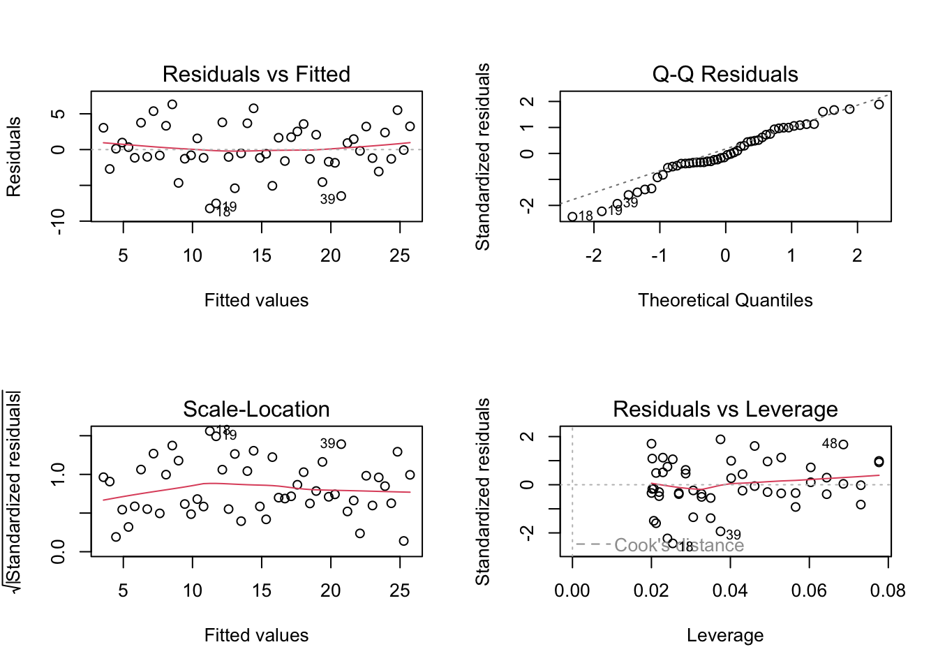
par(mfrow = c(1, 1))A.5.6.8 Common Mistakes in Diagnostics
- Checking only R^2 and ignoring residuals
- Declaring success because p-values are small
- Removing outliers without documenting why
- Ignoring multicollinearity when coefficients are unstable
A.5.6.9 For Logistic Regression and Classification Models
| What to Check | Diagnostic | Problem Signs | If Violated | Chapter |
|---|---|---|---|---|
| Calibration | Calibration plot (observed vs. predicted probabilities) | Predicted probabilities don’t match observed rates | Recalibrate or use different model | 📖 |
| Discrimination | ROC curve, AUC | AUC near 0.5 | Model has no predictive power; add features or try different model | 📖 |
| Influential observations | dfbetas, Cook’s distance analog | Large influence on coefficients | Investigate; consider robust methods | 📖 |
| Goodness of fit | Hosmer-Lemeshow test | Significant p-value | Model doesn’t fit well; consider interactions or nonlinear terms | 📖 |
| Separation | Coefficient estimates very large | Perfect or quasi-separation | Use penalized regression (Firth) or exact methods | 📖 |
A.5.6.10 For Conditional Inference Trees
| What to Check | Diagnostic | Problem Signs | If Violated |
|---|---|---|---|
| Overfitting | Compare training vs. test performance | Large gap between training and test accuracy | Increase mincriterion, prune tree |
| Tree too simple | Only 1-2 terminal nodes | Not capturing real patterns | Decrease mincriterion, check data quality |
| Instability | Different trees from bootstrap samples | Tree structure changes dramatically | Consider ensemble methods (random forest) |
A.5.6.11 Decision: When to Revisit Your Model Choice
Diagnostics reveal problems?
│
├── YES: Assumptions badly violated
│   ├── Try transformation (log, sqrt)
│   ├── Try nonparametric alternative
│   ├── Try robust methods
│   └── Consider different model family
│
├── YES: Poor fit or discrimination
│   ├── Add/remove predictors
│   ├── Add interaction terms
│   ├── Try flexible model (ctree, GAM)
│   └── Collect better data
│
└── NO: Diagnostics look acceptable
    └── Proceed with inference or prediction
Key principle: A model with good diagnostics and moderate fit is more trustworthy than a model with excellent fit but violated assumptions.
Important: Passing diagnostics does not prove a causal relationship; it only supports that the model is not obviously misspecified.
A.5.7 C7: Time Series Models
Time series modeling is for sequential data where observations are ordered in time and typically dependent on previous values. This is fundamentally different from cross-sectional modeling where observations are independent.
When to use time series models instead of regression:
- Data are collected over time at regular intervals
- You want to forecast future values
- Observations are autocorrelated (today’s value depends on yesterday’s)
- There’s trend, seasonality, or other temporal patterns
A.5.7.1 Time Series EDA (before modeling)
Before building a time series model, explore the data using the methods in Table A.4 (Section A2 above).
A.5.7.2 Choosing a Time Series Model
| Situation | Model | When to Use | Chapter | App |
|---|---|---|---|---|
| Simple trend, no seasonality | Exponential smoothing (Holt) | Short-term forecasts, smooth data | 📖 | 🔗 |
| Trend + seasonality | Holt-Winters | Clear seasonal pattern | 📖 | 🔗 |
| Complex autocorrelation | ARIMA | Flexible, handles many patterns | 📖 | 🔗 |
| Seasonal + complex | Seasonal ARIMA (SARIMA) | Seasonal with ARIMA errors | 📖 | 🔗 |
| Known event / structural break | Intervention analysis | ARIMA + pulse/step dummy | 📖 | 🔗 |
| External input influences Y | Transfer function / ARIMAX | Input series available | 📖 | 🔗 |
A.5.7.3 Time Series Model Identification (Box-Jenkins approach)
1. Plot the series → Check for trend, seasonality, variance changes
   │
2. Make stationary → Differencing (d), seasonal differencing (D)
   │                  Transform if variance changes (log, sqrt)
   │
3. Examine ACF/PACF → Identify p, q (and P, Q for seasonal)
   │                   ACF cuts off → MA(q)
   │                   PACF cuts off → AR(p)
   │                   Both decay → ARMA(p,q)
   │
4. Fit model → Estimate parameters
   │
5. Diagnostics → Check residuals (should be white noise)
   │              Ljung-Box test, residual ACF
   │
6. Forecast → Generate predictions with confidence intervals
A.5.7.4 Time Series Diagnostics
After fitting a time series model, check the residuals:
| What to Check | Method | Problem Signs | If Violated |
|---|---|---|---|
| No autocorrelation | Residual ACF, Ljung-Box test | Significant spikes in ACF | Increase model order or add seasonal terms |
| Normality | QQ plot, histogram of residuals | Non-normal shape | May affect confidence intervals |
| Constant variance | Plot residuals over time | Funnel shape, changing spread | Consider GARCH or transformation |
| No pattern | Residuals vs. fitted | Systematic pattern | Model is missing something |
Shiny App: Time Series / ARIMA (includes residual diagnostics)
A.6 Part D: Common Mistakes and How to Avoid Them
A.6.1 Mistake 1: Using the Wrong Test for Your Purpose
Wrong: Using a standard t-test to show two products are equivalent.
A non-significant p-value does NOT prove equivalence — it only means you failed to detect a difference. This could be because there is no difference, OR because your sample was too small.
Right: Use equivalence testing (TOST, Chapter 120) when you want to demonstrate that two things are practically the same.
A.6.2 Mistake 2: Ignoring the Purpose When Evaluating Models
Wrong: Choosing a regression model based on R² when your goal is prediction.
R² measures fit to the training data. A model with high R² might overfit and predict poorly on new data.
Right: For prediction, use cross-validation or a held-out test set to evaluate performance on new data.
A.6.3 Mistake 3: Confusing Description with Inference
Wrong: Calculating a confidence interval when you have the entire population.
If you surveyed all 50 employees in a company, the mean salary is the population mean — there’s nothing to infer.
Right: Confidence intervals and p-values are for inference from samples to populations. If you have the whole population, just report the descriptive statistics.
A.6.4 Mistake 4: Choosing α Without Considering Consequences
Wrong: Always using α = 0.05 because “that’s what everyone does.”
The 5% significance level is arbitrary. In some contexts, 1% is more appropriate; in others, 10% makes sense.
Right: Consider the costs of Type I and Type II errors. Set α to balance these costs appropriately.
A.6.5 Mistake 5: Testing Many Hypotheses Without Correction
Wrong: Testing 20 different relationships and reporting only the significant ones.
With 20 tests at α = 0.05, you expect about 1 false positive by chance alone.
Right: Use multiple testing corrections (Bonferroni, FDR) or pre-register your primary hypothesis.
A.7 Quick Reference Tables
A.7.1 By Research Question
| Question | Method | Requirements | App |
|---|---|---|---|
| Is the mean different from a specific value? | One-sample t-test | Numeric, approximately normal | 🔗 |
| Are two means different? | Two-sample t-test or Welch’s | Numeric, independent groups | 🔗 |
| Are paired measurements different? | Paired t-test | Numeric, matched pairs | 🔗 |
| Are two groups equivalent? | TOST | Numeric, specify equivalence margin | 🔗 |
| Are three or more means different? | ANOVA | Numeric, independent groups | 🔗 |
| Are two categorical variables associated? | Chi-squared test | Categorical, sufficient counts | 🔗 |
| Does data follow a distribution? | K-S test | Continuous data | 🔗 |
| Is there a linear relationship? | Correlation test | Two numeric variables | 🔗 |
| Does X predict Y? | Regression | Depends on Y type | 🔗 |
A.7.2 By Variable Type
| Outcome | Predictor(s) | Method | App |
|---|---|---|---|
| Numeric | None (one group) | One-sample t-test | 🔗 |
| Numeric | Categorical (2 groups) | Two-sample t-test | 🔗 |
| Numeric | Categorical (3+ groups) | ANOVA | 🔗 |
| Numeric | Numeric (1 predictor) | Simple linear regression | 🔗 |
| Numeric | Mixed (multiple) | Multiple linear regression | 🔗 |
| Binary | Mixed | Logistic regression (GLM, binomial) | 🔗 |
| Categorical | Categorical | Chi-squared test | 🔗 |
| Count | Mixed | Poisson regression (GLM, poisson) | 🔗 |
| Time series | Time | ARIMA, exponential smoothing | 🔗 |
For an interactive version of this guide, try the Method Selection Tool — select your constraints (purpose, data type, assumptions) and it will show matching methods.
Use this guide in conjunction with the introductory chapter (Chapter 4) to ensure your statistical analysis matches your research goals.