Generate 50 Random Numbers from an F(20,10) Distribution. Hint: search for the term “Distributions” in RStudio’s help box and click on the link for the F Distribution to find the R command that is needed.
Since there’s no R module available, we write a short script and execute it in RStudio.
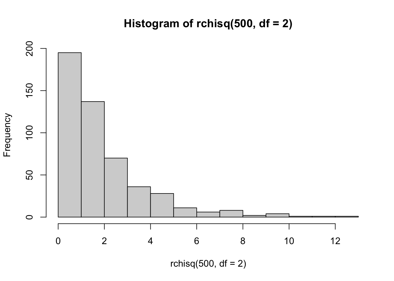
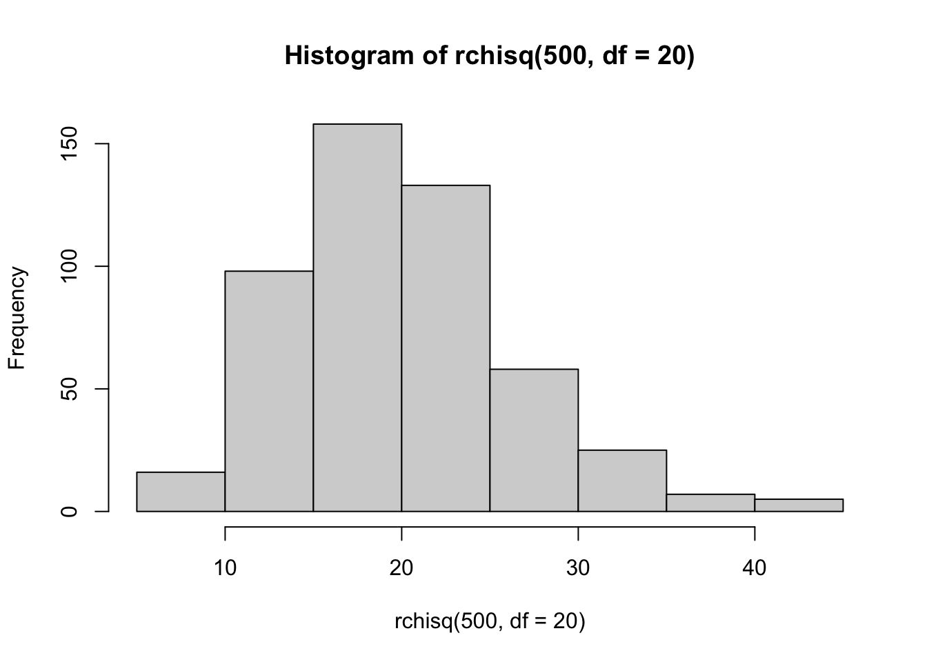
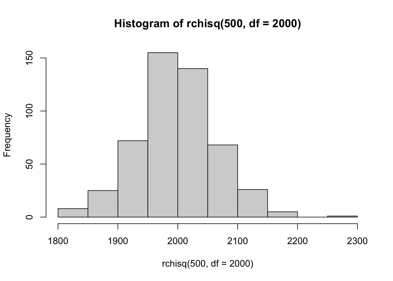
Empirically show that the Histogram of the Chi-squared Density becomes increasingly bell-shaped and resembles a Normal Histogram as the degrees of freedom increase.
We just need to plot Histograms for increasing numbers of degrees of freedom. The third Histogram looks very similar in shape to a Normal Density.
Strictly speaking, convergence to a standard Normal requires standardization: \[
\frac{\chi^2(n)-n}{\sqrt{2n}} \Rightarrow \text{N}(0,1).
\]
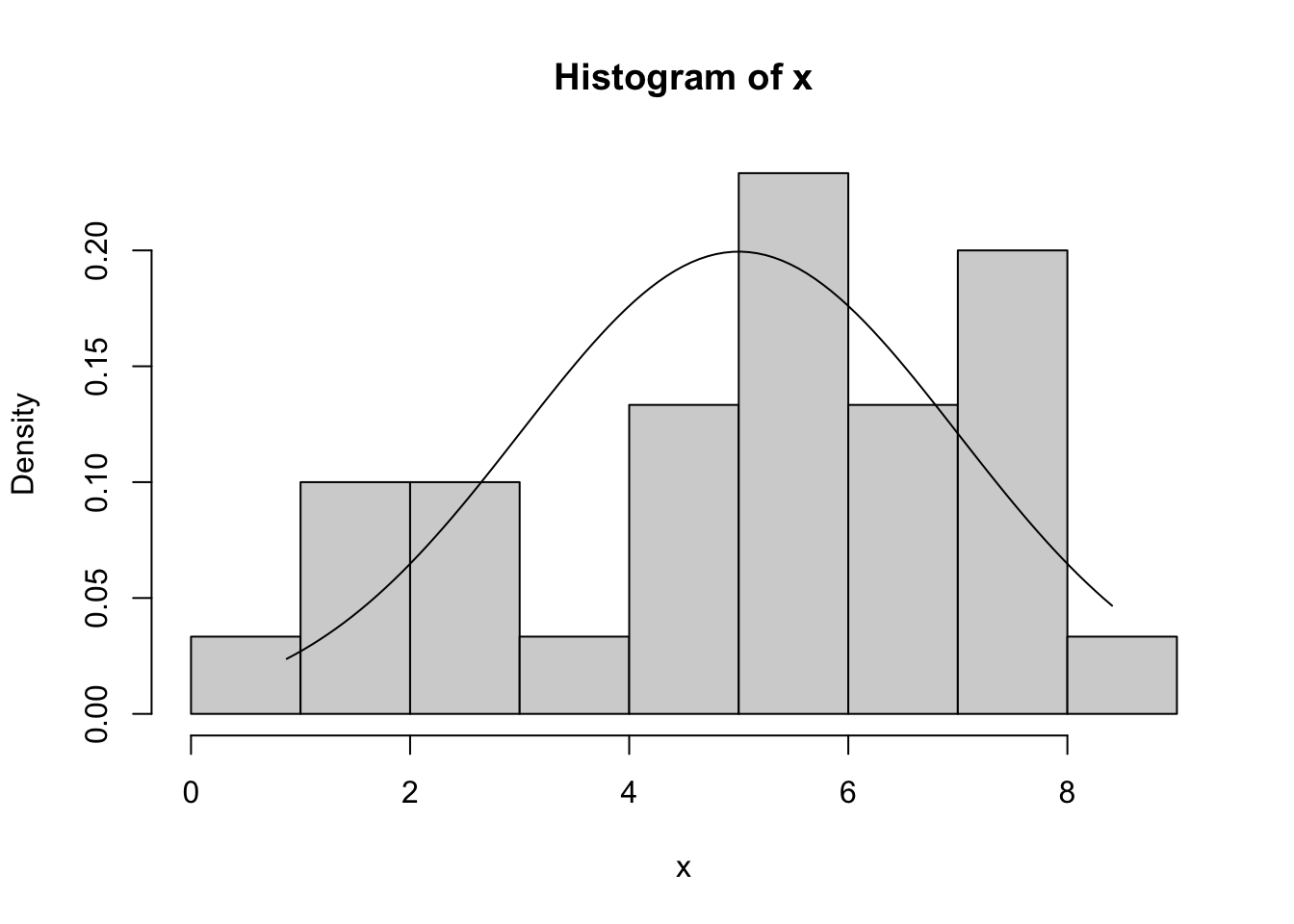
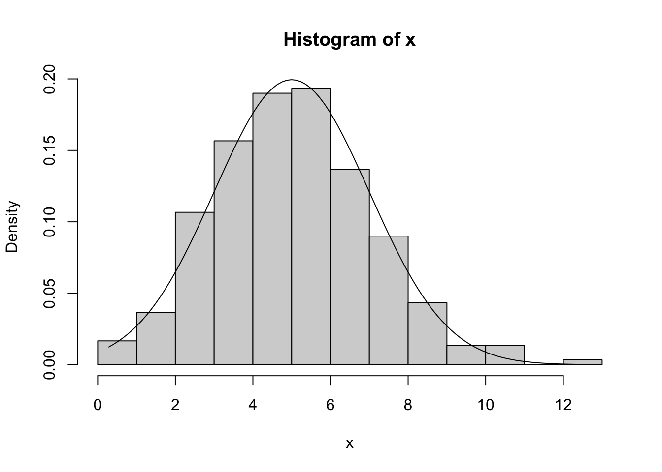
Generate 30 random numbers from the N(5,2) Density function, plot the corresponding Histogram, and overlay the theoretical Density function. Evaluate whether or not the Histogram resembles the theoretical Density.
Repeat the experiment but with 300 observations and comment on what you observe.
To make this solution reproducible, we first set the random seed to 142. After that, we generate random numbers through the rnorm function and display the corresponding Histogram and overlayed curve based of the N(5,2) Density function.
The output clearly illustrates the effect of the Law of Large Numbers from Chapter 10 (the Histogram with 300 random numbers is much closer to the theoretical Density function than with only 30 values).
x =rnorm(300, mean = mymean, sd = mysd)myhist<-hist(x, freq=F)curve(1/(mysd*sqrt(2*pi))*exp(-1/2*((x-mymean)/mysd)^2), min(x), max(x), add=T)
52.2 ML Fitting
The following tasks are based on a spreadsheet which contains simulated distributions: online spreadsheet.
Note: this spreadsheet refreshes random values over time. For strict reproducibility, save a local snapshot (or reproduce the data in R with a fixed set.seed).
Quick intuition: in these tasks, ML fitting and plots are used as screening tools. They help us see whether a candidate distribution is plausible, but they are not formal goodness-of-fit tests. For formal testing procedures and p-value based decisions, see Section 124.1 and Chapter 125 (also summarized in Section 2).
Examine any variable \(U_i\) for \(i = 1, 2, …, 12\) (in columns A:L) and show that it cannot be described well by a Normal Density function. Hint: use the so-called ML Fitting module to do this.
Just copy & paste the values of the chosen column (in the online spreadsheet) into the “Univariate Dataset” text box and observe the output of the analysis. Note: the spreadsheet always updates the random values – therefore, your result will not exactly look identical.
What is the distribution of the data series from Task 4? Use a theoretical argument to answer this question.
The Histogram from Figure that is displayed in the ML Fitting module (see solution of Task 4) is consistent with the fact that the random numbers were generated by a digital computer which typically uses a Uniform Distribution (see Section 19.11).
Show that the data series in column M is approximately normally distributed (based on ML Fitting).
The formula of column M is based on Section 20.22 (i.e. a sum of twelve Uniform variates minus 6). Hence, we expect the data in column M to be approximately normally distributed with \(\mu = 0\) and \(\sigma = 1\).
The ML Fitting method yields the following results (your results may be slightly different):
mean = 0.003791167
standard deviation = 1.028944237
The estimates of both parameters are close to the theoretical values. Due to the Law of Large Numbers, these estimates will get closer to the theoretical values as the number of simulated random numbers increases.
Examine the data in columns N and O. Show that these are not normally distributed and explain (based on theoretical argumentation) why they have a \(\chi^2(n)\) distribution. What is the parameter \(n\)?
The data in columns N and O do not appear to be normally distributed based on the computations found in tab “ML Fitting column N” and “ML Fitting column O”.
The theoretical reason for this is that both columns contain a formula which computes -2 times the natural logarithm of the product of Uniformly distributed variates as is described in Section 23.13. In theory the parameter \(n\) should be equal to 12 (i.e. twice the number of Uniform variates).
If \(Y \sim \text{N}(0,1)\), what is the distribution of \(Y^2\)? Hint: there is a theoretical argument and you can also use the simulated data in column P.
According to theory, the variable \(Y^2 \sim \chi^2(n=1)\) because of Section 23.16. The parameter \(n = 1\) because we only use one normal variate. The ML Fitting method applied to column P can be found in the “ML Fitting column P” tab.
The computation shows that the estimated degrees of freedom is very close to 1 (i.e. the theoretical value). In addition, the Histogram shows that the Chi-squared density function fits the data well.