The Triangular distribution requires only three parameters — a minimum, a maximum, and a most-likely value — making it the practical choice when expert knowledge provides only these three bounds. It is widely used in PERT project scheduling, Monte Carlo simulation, and engineering risk assessment.
Formally, the random variate \(X\) defined for the range \(X \in [a, b]\), is said to have a Triangular Distribution (i.e. \(X \sim \text{Triangular}(a, b, c)\)) with minimum \(a\), maximum \(b\), and mode \(c\), where \(a < c < b\).
40.1 Probability Density Function
\[
f(x) = \begin{cases} \dfrac{2(x-a)}{(b-a)(c-a)} & a \leq x \leq c \\[6pt] \dfrac{2(b-x)}{(b-a)(b-c)} & c < x \leq b \end{cases}
\]
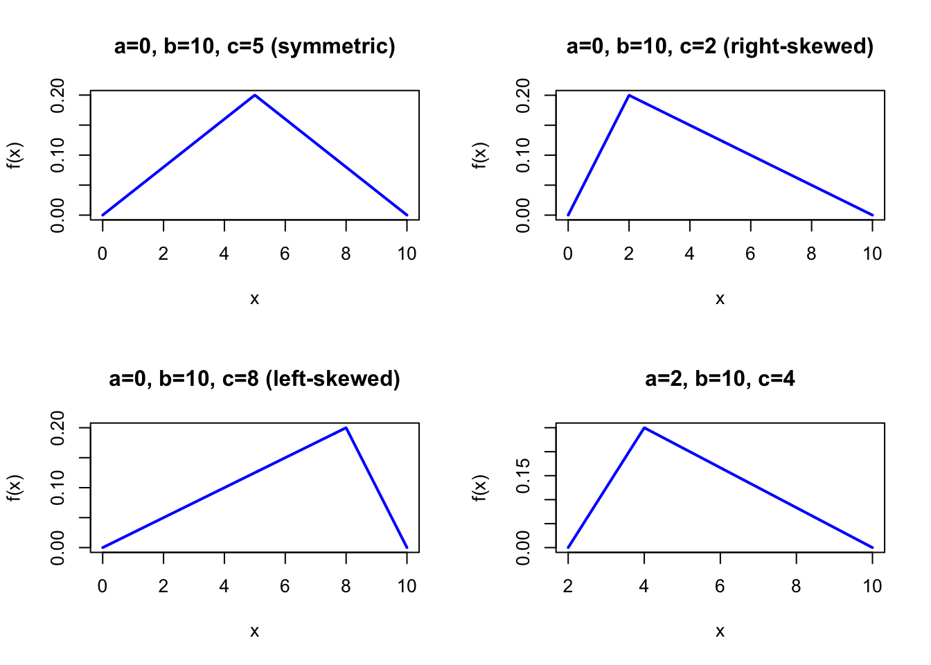
The figure below shows examples of the Triangular Probability Density Function for different parameter combinations.
Code
dtriangular <-function(x, a, b, c) {ifelse(x < a | x > b, 0,ifelse(x <= c,2* (x - a) / ((b - a) * (c - a)),2* (b - x) / ((b - a) * (b - c))))}par(mfrow =c(2, 2))x <-seq(0, 10, length =500)plot(x, dtriangular(x, 0, 10, 5), type ="l", lwd =2, col ="blue",xlab ="x", ylab ="f(x)", main ="a=0, b=10, c=5 (symmetric)")plot(x, dtriangular(x, 0, 10, 2), type ="l", lwd =2, col ="blue",xlab ="x", ylab ="f(x)", main ="a=0, b=10, c=2 (right-skewed)")plot(x, dtriangular(x, 0, 10, 8), type ="l", lwd =2, col ="blue",xlab ="x", ylab ="f(x)", main ="a=0, b=10, c=8 (left-skewed)")x2 <-seq(2, 10, length =500)plot(x2, dtriangular(x2, 2, 10, 4), type ="l", lwd =2, col ="blue",xlab ="x", ylab ="f(x)", main ="a=2, b=10, c=4")par(mfrow =c(1, 1))
Figure 40.1: Triangular Probability Density Function for various parameter combinations
40.2 Purpose
The Triangular distribution is the most widely used distribution in simulation when only expert-elicited bounds and a most-likely value are available. It requires no knowledge of shape or scale parameters beyond what a domain expert can typically estimate. Common applications include:
PERT project scheduling: task duration given optimistic, pessimistic, and most-likely estimates
Monte Carlo simulation when only minimum, maximum, and mode are known
Engineering design: load, strength, and tolerances with known bounds
Financial modeling: revenue and cost estimates from business experts
Supply chain: lead times with lower and upper bounds from supplier data
Relation to the discrete setting. The Triangular distribution is the continuous distribution of the sum of two independent Uniform\((0,1)\) variates, restricted to \([0, 2]\) — analogous to how the discrete triangular distribution (sum of two Discrete Uniform variates) arises. In project scheduling, the discrete analog is a finite probability table over integer task durations.
40.3 Distribution Function
\[
F(x) = \begin{cases} \dfrac{(x-a)^2}{(b-a)(c-a)} & a \leq x \leq c \\[6pt] 1 - \dfrac{(b-x)^2}{(b-a)(b-c)} & c < x \leq b \end{cases}
\]
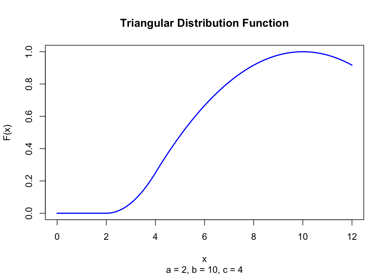
The figure below shows the Triangular Distribution Function for \(a = 2\), \(b = 10\), \(c = 4\).
Code
ptriangular <-function(x, a, b, c) {ifelse(x <= a, 0,ifelse(x <= c, (x - a)^2/ ((b - a) * (c - a)),1- (b - x)^2/ ((b - a) * (b - c))))}x <-seq(0, 12, length =500)plot(x, ptriangular(x, 2, 10, 4), type ="l", lwd =2, col ="blue",xlab ="x", ylab ="F(x)", main ="Triangular Distribution Function",sub ="a = 2, b = 10, c = 4")
Figure 40.2: Triangular Distribution Function (a = 2, b = 10, c = 4)
For the symmetric case \(c = (a+b)/2\): \(g_1 = 0\).
40.17 Coefficient of Kurtosis
\[
g_2 = \frac{12}{5} = 2.4
\]
This is a remarkable fixed constant — the kurtosis is always 2.4, regardless of \(a\), \(b\), and \(c\). The Triangular distribution always has lighter tails than the Normal (\(g_2 = 3\)).
40.18 Parameter Estimation
In practice, parameters are estimated from expert elicitation or sample extremes:
\[
\hat a = x_{(1)}, \quad \hat b = x_{(n)}, \quad \hat c = \text{sample mode estimate}
\]
For simulation purposes, the parameters are typically given directly by domain experts rather than estimated from data.
# Example: verify mean and variance for Triangular(2, 10, 4)a <-2; b <-10; c <-4mean_tri <- (a + b + c) /3var_tri <- (a^2+ b^2+ c^2- a*b - a*c - b*c) /18cat("Mean:", round(mean_tri, 4), "\n")cat("Variance:", round(var_tri, 4), "\n")cat("SD:", round(sqrt(var_tri), 4), "\n")cat("Kurtosis g2:", 12/5, "(always 2.4)\n")
The following code demonstrates Triangular probability calculations:
a <-2; b <-10; c <-4ptriangular <-function(x, a, b, c) {ifelse(x <= a, 0,ifelse(x <= c, (x - a)^2/ ((b - a) * (c - a)),1- (b - x)^2/ ((b - a) * (b - c))))}# P(task <= 5 days)ptriangular(5, a, b, c)# P(task <= mean)ptriangular((a + b + c)/3, a, b, c)# Meancat("Mean:", (a + b + c) /3, "\n")cat("Mode:", c, "\n")
A project task has a minimum duration of \(a = 2\) days, maximum \(b = 10\) days, and most-likely duration \(c = 4\) days: \(X \sim \text{Triangular}(2, 10, 4)\). The expected duration is \((2+10+4)/3 \approx 5.33\) days.
a <-2; b <-10; c <-4ptriangular <-function(x, a, b, c) {ifelse(x <= a, 0,ifelse(x <= c, (x - a)^2/ ((b - a) * (c - a)),1- (b - x)^2/ ((b - a) * (b - c))))}# Expected durationcat("Expected duration (days):", (a + b + c) /3, "\n")# P(task done within 5 days)cat("P(done within 5 days):", round(ptriangular(5, a, b, c), 4), "\n")# P(task takes more than 8 days)cat("P(takes > 8 days):", round(1-ptriangular(8, a, b, c), 4), "\n")
The kurtosis \(g_2 = 12/5 = 2.4\) is always fixed, regardless of \(a\), \(b\), and \(c\). This means the Triangular distribution is always platykurtic (lighter-tailed than the Normal), which follows from the bounded support.
40.23 Property 2: Symmetric Special Case
When \(c = (a+b)/2\) the distribution is symmetric (\(g_1 = 0\)) and resembles a tent function. The Uniform distribution is not the limit of this case — the symmetric Triangular distribution retains its triangular density.
40.24 Property 3: Sum of Two Uniforms
The Triangular\((0, 2, 1)\) distribution is the distribution of the sum of two independent Uniform\((0,1)\) random variables. More generally, Triangular\((a, b, (a+b)/2)\) arises as a scaled and shifted sum of two Uniforms.
40.25 Related Distributions 1: Uniform Distribution
The Uniform distribution on \([a, b]\) is the limiting case when all three parameters \(a, c, b\) provide equal weight (flat density, \(c\) varies), and when \(a=b=c\) would be degenerate. The Triangular is a first-order improvement over the Uniform when expert knowledge about the most-likely value is available (see Chapter 19).