46  Frechet Distribution

The Frechet distribution is the extreme-value distribution for block maxima drawn from heavy-tailed parent distributions. When the underlying data follow a Pareto, Student-\(t\), Cauchy, or any regularly varying distribution, the normalized maximum converges to a Frechet distribution, making it the canonical model for extreme events with potentially unbounded severity.

Formally, the random variate \(X\) defined for the range \(X > m\), is said to have a Frechet Distribution (i.e. \(X \sim \text{Frechet}(\alpha, s, m)\)) with shape parameter \(\alpha > 0\), scale parameter \(s > 0\), and location parameter \(m \geq 0\). The Frechet distribution is also known as the GEV Type II distribution or the inverse Weibull distribution (for maxima). We define \(z = (x - m)/s\) throughout this chapter.

46.1 Probability Density Function

\[ f(x) = \frac{\alpha}{s}\left(\frac{x - m}{s}\right)^{-1-\alpha}\exp\!\left(-\left(\frac{x - m}{s}\right)^{-\alpha}\right), \quad x > m \]

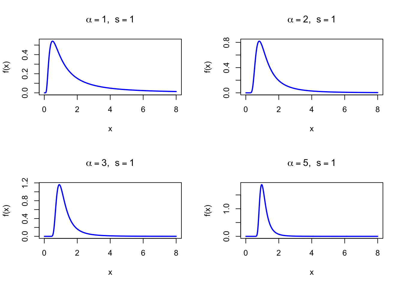
The figure below shows examples of the Frechet Probability Density Function for different shape values with \(s = 1\) and \(m = 0\).

dfrechet <- function(x, alpha, s = 1, m = 0) {
  z <- (x - m) / s
  valid <- z > 0
  d <- rep(0, length(x))
  d[valid] <- (alpha / s) * z[valid]^(-1 - alpha) * exp(-z[valid]^(-alpha))
  d
}

par(mfrow = c(2, 2))
x <- seq(0.01, 8, length = 500)

plot(x, dfrechet(x, 1), type = "l", lwd = 2, col = "blue",
     xlab = "x", ylab = "f(x)", main = expression(paste(alpha == 1, ",  ", s == 1)))

plot(x, dfrechet(x, 2), type = "l", lwd = 2, col = "blue",
     xlab = "x", ylab = "f(x)", main = expression(paste(alpha == 2, ",  ", s == 1)))

plot(x, dfrechet(x, 3), type = "l", lwd = 2, col = "blue",
     xlab = "x", ylab = "f(x)", main = expression(paste(alpha == 3, ",  ", s == 1)))

plot(x, dfrechet(x, 5), type = "l", lwd = 2, col = "blue",
     xlab = "x", ylab = "f(x)", main = expression(paste(alpha == 5, ",  ", s == 1)))

par(mfrow = c(1, 1))

Figure 46.1: Frechet Probability Density Function for various shape values (scale = 1, location = 0)

46.2 Purpose

The Frechet distribution arises as the limiting distribution of block maxima from heavy-tailed parent distributions, whose survival function decays as a power law. Its defining characteristic is a polynomially decaying right tail, which assigns substantially more probability to extreme outcomes than light-tailed models such as the Gumbel. Common applications include:

• Extreme financial losses: modeling the largest daily portfolio losses or maximum drawdowns
• Catastrophic insurance claims: annual maximum claim sizes in reinsurance
• Extreme pollution concentrations: maximum pollutant levels from industrial incidents
• Telecommunications traffic peaks: maximum data throughput or congestion events
• Extreme precipitation: maximum rainfall intensities in heavy-tailed climatic regimes

Relation to the discrete setting. The Frechet distribution is the continuous limit of the maximum of \(n\) i.i.d. random variables from heavy-tailed parents. In the discrete domain, the normalized maximum of regularly varying discrete distributions (e.g., Zipf, Yule-Simon) also converges to the Frechet distribution after appropriate normalization.

46.3 Distribution Function

\[ F(x) = \exp\!\left(-\left(\frac{x - m}{s}\right)^{-\alpha}\right), \quad x > m \]

In R (using the evd package): pfrechet(x, loc = m, scale = s, shape = alpha).

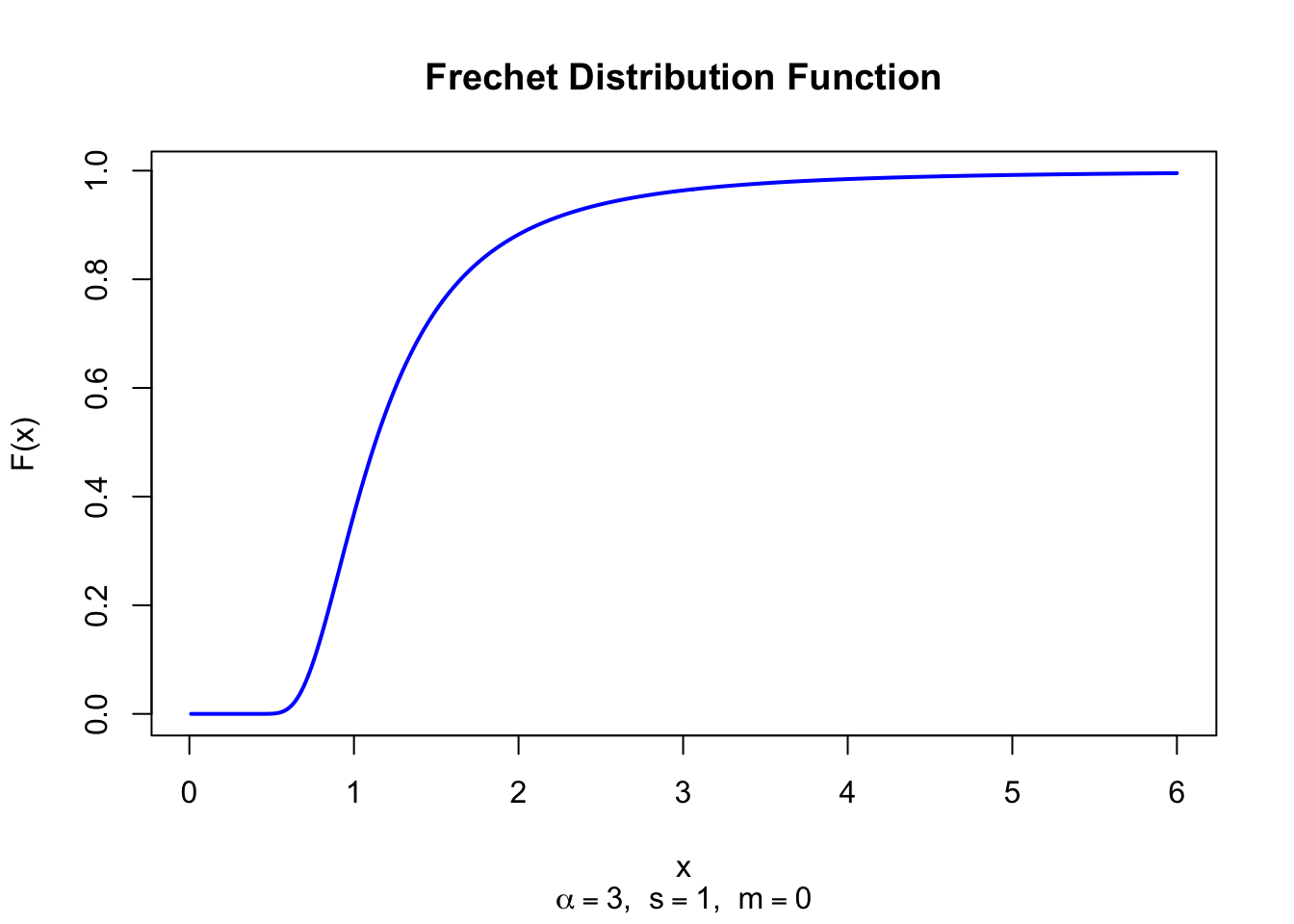
The figure below shows the Frechet Distribution Function for \(\alpha = 3\), \(s = 1\), and \(m = 0\).

pfrechet <- function(x, alpha, s = 1, m = 0) {
  z <- (x - m) / s
  valid <- z > 0
  p <- rep(0, length(x))
  p[valid] <- exp(-z[valid]^(-alpha))
  p
}

x <- seq(0.01, 6, length = 500)
plot(x, pfrechet(x, 3), type = "l", lwd = 2, col = "blue",
     xlab = "x", ylab = "F(x)", main = "Frechet Distribution Function",
     sub = expression(paste(alpha == 3, ",  ", s == 1, ",  ", m == 0)))

Figure 46.2: Frechet Distribution Function (shape = 3, scale = 1, location = 0)

46.4 Moment Generating Function

The moment generating function of the Frechet distribution does not exist in closed form because the heavy right tail causes \(E[e^{tX}]\) to diverge for all \(t > 0\).

Raw moments are expressed in terms of the gamma function:

\[ E\!\left[(X - m)^n\right] = s^n\,\Gamma\!\left(1 - \frac{n}{\alpha}\right), \quad n < \alpha \]

46.5 1st Uncentered Moment

\[ \mu_1' = m + s\,\Gamma\!\left(1 - \frac{1}{\alpha}\right), \quad \alpha > 1 \]

For \(\alpha \leq 1\), the mean is infinite.

46.6 2nd Uncentered Moment

\[ \mu_2' = m^2 + 2ms\,\Gamma\!\left(1 - \frac{1}{\alpha}\right) + s^2\,\Gamma\!\left(1 - \frac{2}{\alpha}\right), \quad \alpha > 2 \]

46.7 3rd Uncentered Moment

\[ \mu_3' = m^3 + 3m^2 s\,\Gamma\!\left(1-\frac{1}{\alpha}\right) + 3ms^2\,\Gamma\!\left(1-\frac{2}{\alpha}\right) + s^3\,\Gamma\!\left(1-\frac{3}{\alpha}\right), \quad \alpha > 3 \]

46.8 4th Uncentered Moment

\[ \mu_4' = m^4 + 4m^3 s\,\Gamma\!\left(1-\frac{1}{\alpha}\right) + 6m^2 s^2\,\Gamma\!\left(1-\frac{2}{\alpha}\right) + 4ms^3\,\Gamma\!\left(1-\frac{3}{\alpha}\right) + s^4\,\Gamma\!\left(1-\frac{4}{\alpha}\right), \quad \alpha > 4 \]

46.9 2nd Centered Moment

\[ \mu_2 = s^2\!\left[\Gamma\!\left(1 - \frac{2}{\alpha}\right) - \Gamma\!\left(1 - \frac{1}{\alpha}\right)^2\right], \quad \alpha > 2 \]

46.10 3rd Centered Moment

\[ \mu_3 = s^3\!\left[\Gamma\!\left(1 - \frac{3}{\alpha}\right) - 3\,\Gamma\!\left(1 - \frac{2}{\alpha}\right)\Gamma\!\left(1 - \frac{1}{\alpha}\right) + 2\,\Gamma\!\left(1 - \frac{1}{\alpha}\right)^3\right], \quad \alpha > 3 \]

46.11 4th Centered Moment

\[ \mu_4 = s^4\!\left[\Gamma\!\left(1 - \frac{4}{\alpha}\right) - 4\,\Gamma\!\left(1 - \frac{3}{\alpha}\right)\Gamma\!\left(1 - \frac{1}{\alpha}\right) + 6\,\Gamma\!\left(1 - \frac{2}{\alpha}\right)\Gamma\!\left(1 - \frac{1}{\alpha}\right)^2 - 3\,\Gamma\!\left(1 - \frac{1}{\alpha}\right)^4\right], \quad \alpha > 4 \]

46.12 Expected Value

\[ \text{E}(X) = m + s\,\Gamma\!\left(1 - \frac{1}{\alpha}\right), \quad \alpha > 1 \]

For \(\alpha \leq 1\), the expected value is infinite — the distribution has such a heavy tail that the average does not converge.

46.13 Variance

\[ \text{V}(X) = s^2\!\left[\Gamma\!\left(1 - \frac{2}{\alpha}\right) - \Gamma\!\left(1 - \frac{1}{\alpha}\right)^2\right], \quad \alpha > 2 \]

For \(\alpha \leq 2\), the variance is infinite.

46.14 Median

\[ \text{Med}(X) = m + \frac{s}{(\ln 2)^{1/\alpha}} \]

The median always exists regardless of \(\alpha\), unlike the mean and variance.

46.15 Mode

\[ \text{Mo}(X) = m + s\left(\frac{\alpha}{\alpha + 1}\right)^{1/\alpha} \]

The mode always exists and lies between the location \(m\) and the median.

46.16 Coefficient of Skewness

\[ g_1 = \frac{\Gamma(1-3/\alpha) - 3\,\Gamma(1-2/\alpha)\,\Gamma(1-1/\alpha) + 2\,\Gamma(1-1/\alpha)^3}{\bigl[\Gamma(1-2/\alpha) - \Gamma(1-1/\alpha)^2\bigr]^{3/2}}, \quad \alpha > 3 \]

The skewness is always positive and increases as \(\alpha\) decreases (heavier tail). For \(\alpha \leq 3\), the skewness is undefined because the third moment does not exist.

46.17 Coefficient of Kurtosis

\[ g_2 = \frac{\Gamma(1-4/\alpha) - 4\,\Gamma(1-3/\alpha)\,\Gamma(1-1/\alpha) + 6\,\Gamma(1-2/\alpha)\,\Gamma(1-1/\alpha)^2 - 3\,\Gamma(1-1/\alpha)^4}{\bigl[\Gamma(1-2/\alpha) - \Gamma(1-1/\alpha)^2\bigr]^{2}}, \quad \alpha > 4 \]

For \(\alpha \leq 4\), the kurtosis is undefined. When it exists, the kurtosis exceeds 3 (leptokurtic), reflecting the heavy tail.

46.18 Parameter Estimation

Maximum likelihood estimation is the standard approach. The log-likelihood for a sample \(x_1, \ldots, x_n\) (with known \(m = 0\)) is:

\[ \ell(\alpha, s) = n\ln\alpha - n\ln s - (1+\alpha)\sum_{i=1}^n \ln\!\left(\frac{x_i}{s}\right) - \sum_{i=1}^n \left(\frac{x_i}{s}\right)^{-\alpha} \]

In R, the evd package provides fgev() with the parameterization \(\xi = 1/\alpha\), or one can use fitdistr() with a custom density.

library(evd)

set.seed(42)
alpha_true <- 3; s_true <- 2; m_true <- 0
# GEV with xi = 1/alpha, scale = s * xi, loc = m + s * (1 - xi^(-xi)) ...
# Direct simulation via inverse CDF
u <- runif(200)
x_obs <- m_true + s_true * (-log(u))^(-1/alpha_true)

# Fit GEV (xi = 1/alpha for Frechet)
fit <- fgev(x_obs)
xi_hat <- fit$estimate["shape"]
sigma_hat <- fit$estimate["scale"]
mu_hat <- fit$estimate["loc"]

# Convert to Frechet parameterization
alpha_hat <- 1 / xi_hat
s_hat <- sigma_hat / xi_hat
m_hat <- mu_hat - s_hat

cat("MLE alpha:", round(alpha_hat, 4), "\n")
cat("MLE s:    ", round(s_hat, 4), "\n")
cat("MLE m:    ", round(m_hat, 4), "\n")
cat("True alpha:", alpha_true, "  True s:", s_true, "  True m:", m_true, "\n")

MLE alpha: 4.962 
MLE s:     3.7535 
MLE m:     -1.671 
True alpha: 3   True s: 2   True m: 0 

46.19 R Module

46.19.1 RFC

The Frechet Distribution module is available in RFC under the menu “Distributions / Frechet Distribution”.

46.19.2 Direct app link

• https://shiny.wessa.net/frechet/

46.19.3 R Code

The following code demonstrates Frechet probability calculations using custom functions and the evd package:

library(evd)

alpha <- 3; s <- 2; m <- 0

# Custom density
dfrechet <- function(x, alpha, s, m) {
  z <- (x - m) / s
  (alpha / s) * z^(-1 - alpha) * exp(-z^(-alpha))
}

# Custom CDF
pfrechet <- function(x, alpha, s, m) {
  exp(-((x - m) / s)^(-alpha))
}

# Probability density at x = 3
dfrechet(3, alpha, s, m)

# Distribution function: P(X <= 3)
pfrechet(3, alpha, s, m)

# Quantile function: median
qfrechet(0.5, loc = m, scale = s, shape = alpha)

# Mean and mode
cat("Mean:", m + s * gamma(1 - 1/alpha), "\n")
cat("Mode:", m + s * (alpha / (alpha + 1))^(1/alpha), "\n")
cat("Median:", m + s / (log(2))^(1/alpha), "\n")

# Generate random Frechet numbers
set.seed(42)
rfrechet(10, loc = m, scale = s, shape = alpha)

[1] 0.2203162
[1] 0.7435671
[1] 2.259895
Mean: 2.708236 
Mode: 1.817121 
Median: 2.259895 
 [1] 3.429485 2.296073 3.044506 5.938903 2.566584 1.761516 2.942573 2.691884
 [9] 1.886485 2.236776

46.20 Example

An insurance company models its annual maximum claim size (in millions of euros) as \(X \sim \text{Frechet}(\alpha = 3, s = 2, m = 0)\). The shape \(\alpha = 3\) implies heavy tails: the mean exists (\(\alpha > 1\)) and the variance exists (\(\alpha > 2\)), but the skewness is only marginally defined (\(\alpha = 3\)). We compute key risk metrics.

library(evd)

alpha <- 3; s <- 2; m <- 0

# Custom CDF
pfrechet_custom <- function(x, alpha, s, m) exp(-((x - m) / s)^(-alpha))

# P(max claim > 5 million)
cat("P(max claim > 5M):", 1 - pfrechet_custom(5, alpha, s, m), "\n")

# Mean annual maximum claim
cat("Mean max claim (M EUR):", m + s * gamma(1 - 1/alpha), "\n")

# Median annual maximum claim
cat("Median max claim (M EUR):", round(m + s / (log(2))^(1/alpha), 4), "\n")

# 100-year return level (99th percentile)
rl_100 <- qfrechet(0.99, loc = m, scale = s, shape = alpha)
cat("100-year return level (M EUR):", round(rl_100, 2), "\n")

# 50-year return level (98th percentile)
rl_50 <- qfrechet(0.98, loc = m, scale = s, shape = alpha)
cat("50-year return level (M EUR):", round(rl_50, 2), "\n")

P(max claim > 5M): 0.061995 
Mean max claim (M EUR): 2.708236 
Median max claim (M EUR): 2.2599 
100-year return level (M EUR): 9.27 
50-year return level (M EUR): 7.34 

Interactive Shiny app (click to load).

Open in new tab

46.21 Random Number Generator

Frechet random variates are generated via the inverse-CDF method. Since \(F(x) = \exp\!\bigl(-((x-m)/s)^{-\alpha}\bigr)\), solving \(U = F(X)\) for \(X\) gives:

\[ X = m + s\,(-\ln U)^{-1/\alpha} \sim \text{Frechet}(\alpha, s, m) \quad \text{when } U \sim \text{U}(0,1) \]

set.seed(123)
n <- 1000; alpha <- 3; s <- 2; m <- 0

# Inverse-transform method
u <- runif(n)
x_inv <- m + s * (-log(u))^(-1/alpha)

cat("Simulated mean:", round(mean(x_inv), 4), "\n")
cat("Theoretical mean:", round(m + s * gamma(1 - 1/alpha), 4), "\n")
cat("Simulated var:", round(var(x_inv), 4), "\n")
theo_var <- s^2 * (gamma(1 - 2/alpha) - gamma(1 - 1/alpha)^2)
cat("Theoretical var:", round(theo_var, 4), "\n")

Simulated mean: 2.6759 
Theoretical mean: 2.7082 
Simulated var: 2.4917 
Theoretical var: 3.3812 

Interactive Shiny app (click to load).

Open in new tab

46.22 Property 1: Special Case of GEV with Positive Shape

The Frechet\((\alpha, s, m)\) distribution is a GEV distribution with shape \(\xi = 1/\alpha > 0\). Specifically, if \(X \sim \text{Frechet}(\alpha, s, m)\), then:

\[ X \sim \text{GEV}\!\left(\mu = m + s,\; \sigma = \frac{s}{\alpha},\; \xi = \frac{1}{\alpha}\right) \]

See Chapter 45.

46.23 Property 2: Domain of Attraction

The Frechet distribution arises as the limit for the maximum of i.i.d. random variables from heavy-tailed (regularly varying) distributions. A distribution \(F\) belongs to the Frechet domain of attraction if and only if:

\[ \lim_{x \to \infty} \frac{1 - F(tx)}{1 - F(x)} = t^{-\alpha}, \quad t > 0 \]

Examples of distributions in this domain: Pareto, Student-\(t\), Cauchy, Burr, and Log-Gamma.

46.24 Property 3: Power-Law Tail

The survival function of the Frechet distribution decays as a power law for large \(x\):

\[ 1 - F(x) \sim \left(\frac{x - m}{s}\right)^{-\alpha} \quad \text{as } x \to \infty \]

This means the Frechet tail is Pareto-like: for large \(x\), the tail probability decreases polynomially rather than exponentially, assigning substantial probability to extreme outcomes.

46.25 Property 4: Reciprocal Weibull Relationship

If \(X \sim \text{Frechet}(\alpha, 1, 0)\) then \(1/X \sim \text{Weibull}(\alpha, 1)\). More generally:

\[ X \sim \text{Frechet}(\alpha, s, 0) \quad \Longleftrightarrow \quad \frac{s}{X} \sim \text{Weibull}(\alpha, 1) \]

This duality connects the extreme-value distribution for maxima (Frechet) to the extreme-value distribution for minima (Weibull).

46.26 Related Distributions 1: GEV Distribution

The Frechet distribution is the GEV distribution with \(\xi > 0\). Fitting a GEV and finding \(\hat\xi > 0\) is equivalent to finding Frechet-type extreme-value behavior (see Chapter 45).

46.27 Related Distributions 2: Pareto Distribution

The Pareto distribution belongs to the Frechet domain of attraction. For large \(x\), the Frechet and Pareto tails are asymptotically equivalent. The Frechet is the extreme-value version of the Pareto (see Chapter 32).

46.28 Related Distributions 3: Gumbel Distribution

The Gumbel distribution is the GEV with \(\xi = 0\), corresponding to light-tailed parents. As \(\alpha \to \infty\) (equivalently \(\xi \to 0\)), the Frechet distribution approaches the Gumbel (see Chapter 38).

46.29 Related Distributions 4: Weibull Distribution

The Weibull distribution is connected to the Frechet distribution via the reciprocal transformation \(1/X\). The reversed Weibull (\(\xi < 0\) in GEV) models bounded-tail extremes, complementing the unbounded Frechet distribution (see Chapter 31).