Kernel Density Estimation (Rosenblatt 1956; Parzen 1962) is a non-parametric method for estimating the probability density function of a random variable. If \((x_1, x_2, …, x_n)\) is an independently and identically distributed sample from any density function \(f\) then the Kernel Density Estimator is
where \(K_h()\) is the Kernel function with bandwidth \(h > 0\). The function \(K_h(z) \geq 0\) and has a unit integral \(\left( \int_\mathbb{R} K_h(z)\text{d}z = 1 \right)\) and a mean of 0. In other words, each sample point \(x_i\) is replaced by a Kernel function and the estimated Kernel Density is equal to the sum of all the Kernel functions.
80.1.1 Horizontal axis of the Kernel Density Plot
The horizontal axis represents the values of the variable under investigation.
80.1.2 Vertical axis of the Kernel Density Plot
The vertical axis represents the estimated density.
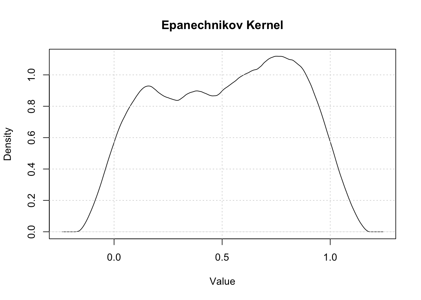
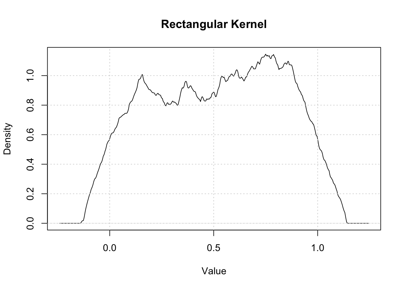
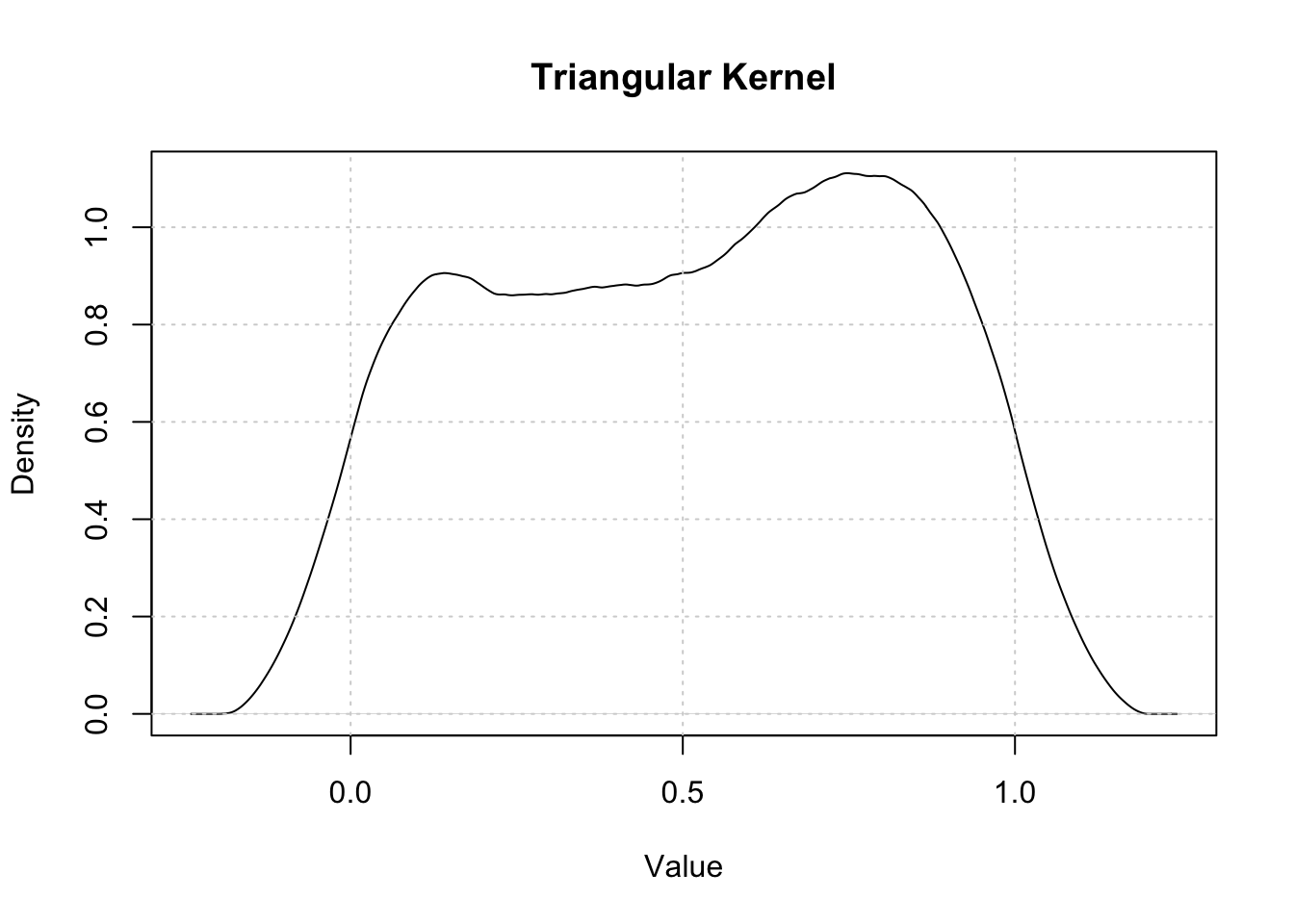
To compute the Kernel Density Plot, the R code uses the density function with a parameter that defines the bandwidth and another parameter for the kernel.
80.9 Purpose
The Kernel Density Plot is used to visualize the empirical density of the variable under investigation. Sometimes the Kernel Densities are used to transform the data before computing some statistic which is used in subsequent analysis. The transformation which is induced can be interpreted as having a smoothing effect.
80.10 Bandwidth Selection
The bandwidth \(h\) controls the smoothness of the estimated density:
small \(h\): more detail, but noisier estimates (higher variance)
large \(h\): smoother estimates, but potentially oversmoothed (higher bias)
In practice, software often uses a default rule such as Silverman’s rule of thumb (Silverman 1986) or similar plug-in rules. These defaults are usually reasonable as a starting point, but it is good practice to inspect how conclusions change under slightly smaller and larger bandwidths.
80.11 Pros & Cons
80.11.1 Pros
The Kernel Density Plot has the following advantages:
Unlike the Histogram, it does not require to specify the number of bins.
It is easily interpreted and provides a lot of (detailed) information about the empirical density function.
80.11.2 Cons
The Kernel Density Plot has the following disadvantages:
It requires a bandwidth parameter to be specified. In most cases, however, the software will use a fairly appropriate bandwidth.
Not all software packages allow the computation of the Kernel Density Plot.
The analysis shows the Gaussian Kernel Density Plot for the monthly marriages time series. It can be concluded that the time series exhibits a “camel shape” which indicates a bimodal density (there are two local maxima). The left hump of the camel shape is higher than the right one -- this implies that the left hump is displayed in the Table as a “global” maximum.
80.13 Task
Try to explain why the marriages time series is bimodal. Also, compare this result with the Kernel Density Plot for the monthly divorces time series (same country, same period). Why do both time series seem to have different distributions?
Epanechnikov, V. A. 1969. “Non-Parametric Estimation of a Multivariate Probability Density.”Theory of Probability and Its Applications 14 (1): 153–58. https://doi.org/10.1137/1114019.
Parzen, Emanuel. 1962. “On Estimation of a Probability Density Function and Mode.”The Annals of Mathematical Statistics 33 (3): 1065–76. https://doi.org/10.1214/aoms/1177704472.
Rosenblatt, Murray. 1956. “Remarks on Some Nonparametric Estimates of a Density Function.”The Annals of Mathematical Statistics 27 (3): 832–37. https://doi.org/10.1214/aoms/1177728190.
Silverman, B. W. 1986. Density Estimation for Statistics and Data Analysis. London: Chapman; Hall.