The Laplace distribution — also called the double Exponential — consists of two Exponential tails joined at a central point. It is the distribution that minimizes the expected absolute deviation (rather than squared deviation), making it the natural model for data with frequent large deviations and for L1 (least-absolute-deviations) regression.
Formally, the random variate \(X\) defined for all of \(\mathbb{R}\), is said to have a Laplace Distribution (i.e. \(X \sim \text{Laplace}(\mu, b)\)) with location parameter \(\mu \in \mathbb{R}\) and scale parameter \(b > 0\). The Laplace distribution is not built into base R; custom density and distribution functions are used.
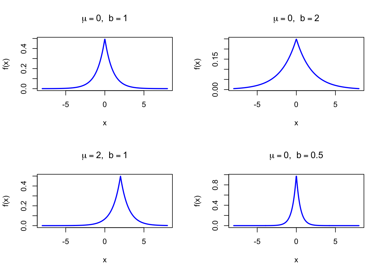
The figure below shows examples of the Laplace Probability Density Function for different parameter combinations.
Code
dlaplace <-function(x, mu, b) {exp(-abs(x - mu) / b) / (2* b)}par(mfrow =c(2, 2))x <-seq(-8, 8, length =500)plot(x, dlaplace(x, 0, 1), type ="l", lwd =2, col ="blue",xlab ="x", ylab ="f(x)", main =expression(paste(mu ==0, ", ", b ==1)))plot(x, dlaplace(x, 0, 2), type ="l", lwd =2, col ="blue",xlab ="x", ylab ="f(x)", main =expression(paste(mu ==0, ", ", b ==2)))plot(x, dlaplace(x, 2, 1), type ="l", lwd =2, col ="blue",xlab ="x", ylab ="f(x)", main =expression(paste(mu ==2, ", ", b ==1)))plot(x, dlaplace(x, 0, 0.5), type ="l", lwd =2, col ="blue",xlab ="x", ylab ="f(x)", main =expression(paste(mu ==0, ", ", b ==0.5)))par(mfrow =c(1, 1))
Figure 37.1: Laplace Probability Density Function for various parameter combinations
37.2 Purpose
The Laplace distribution is the double-sided Exponential — it places equal-weight Exponential tails on both sides of the location parameter. Because it minimizes the mean absolute error (MAE) rather than the mean squared error, its MLE corresponds to the sample median rather than the mean. Common applications include:
Financial daily returns and log-price changes (heavier tails than Normal)
Sparse signal recovery and LASSO regularization (Laplace prior on coefficients)
Image processing: modeling wavelet coefficients which tend to be sparse
Robust statistics: less sensitive to outliers than the Normal distribution
Relation to the discrete setting. The Laplace is a double-sided Exponential; since the Exponential is the continuous analog of the Geometric distribution, the Laplace is the continuous analog of the discrete Laplace distribution (also called the bilateral geometric distribution), defined as the difference of two i.i.d. Geometric variates.
37.3 Distribution Function
\[
F(x) = \begin{cases} \dfrac{1}{2}\exp\!\left(\dfrac{x-\mu}{b}\right) & x \leq \mu \\[6pt] 1 - \dfrac{1}{2}\exp\!\left(-\dfrac{x-\mu}{b}\right) & x > \mu \end{cases}
\]
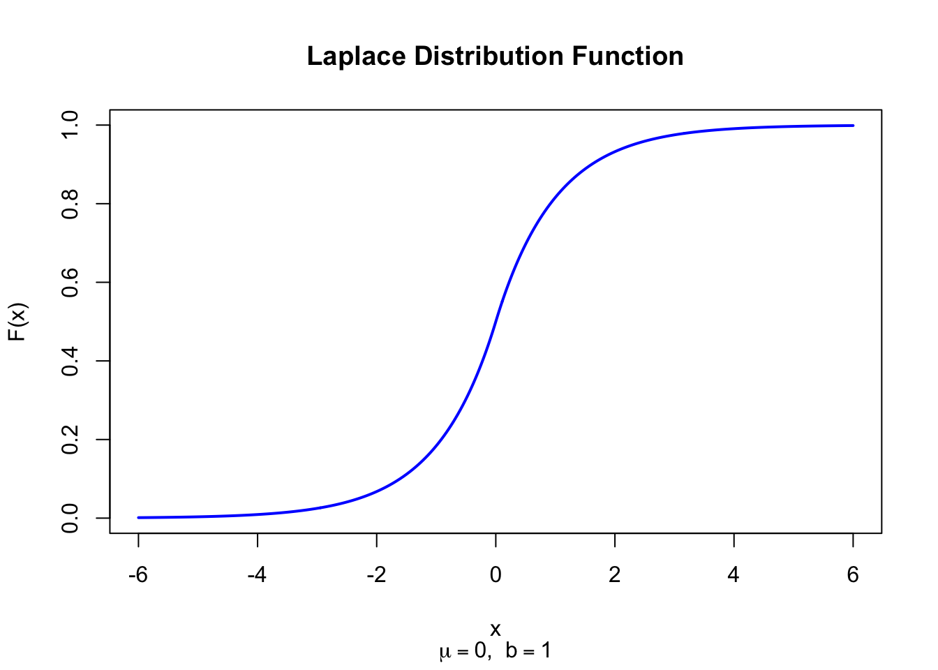
The figure below shows the Laplace Distribution Function for \(\mu = 0\) and \(b = 1\).
Code
plaplace <-function(x, mu, b) {ifelse(x <= mu,0.5*exp((x - mu) / b),1-0.5*exp(-(x - mu) / b))}x <-seq(-6, 6, length =500)plot(x, plaplace(x, 0, 1), type ="l", lwd =2, col ="blue",xlab ="x", ylab ="F(x)", main ="Laplace Distribution Function",sub =expression(paste(mu ==0, ", ", b ==1)))
Figure 37.2: Laplace Distribution Function (location = 0, scale = 1)
The following code demonstrates Laplace probability calculations:
mu <-0; b <-2dlaplace <-function(x, mu, b) exp(-abs(x - mu) / b) / (2* b)plaplace <-function(x, mu, b) {ifelse(x <= mu, 0.5*exp((x - mu)/b), 1-0.5*exp(-(x - mu)/b))}# Density at x = 0dlaplace(0, mu, b)# P(|X| > 4): both tails beyond 41-plaplace(4, mu, b) +plaplace(-4, mu, b)# Mean and SDcat("Mean:", mu, "\n")cat("SD:", sqrt(2) * b, "\n")
[1] 0.25
[1] 0.1353353
Mean: 0
SD: 2.828427
37.20 Example
Daily financial log-returns are modeled as \(X \sim \text{Laplace}(\mu = 0, b = 2)\). The probability that the absolute return exceeds 4 is \(e^{-2} \approx 0.135\).
mu <-0; b <-2plaplace <-function(x, mu, b) {ifelse(x <= mu, 0.5*exp((x - mu)/b), 1-0.5*exp(-(x - mu)/b))}# P(|return| > 4)p_tail <-2* (1-plaplace(4, mu, b))cat("P(|return| > 4):", round(p_tail, 6), "\n")cat("Exact value exp(-2):", exp(-2), "\n")# Compare with Normal having same variancesigma_norm <-sqrt(2) * bp_norm <-2*pnorm(-4, 0, sigma_norm)cat("Same under Normal:", round(p_norm, 6), "\n")
P(|return| > 4): 0.135335
Exact value exp(-2): 0.1353353
Same under Normal: 0.157299
If \(Y_1, Y_2 \overset{\text{i.i.d.}}{\sim} \text{Exp}(1)\) then:
\[
X = \mu + b(Y_1 - Y_2) \sim \text{Laplace}(\mu, b)
\]
This construction confirms the interpretation as a “double Exponential” and provides an alternative random number generator.
37.23 Property 2: L1 MLE
Maximizing the Laplace log-likelihood is equivalent to minimizing \(\sum|x_i - \mu|\), so the MLE of \(\mu\) is the sample median rather than the mean. This is the basis of L1 (least absolute deviations) regression.
37.24 Property 3: Kurtosis
The kurtosis \(g_2 = 6\) (excess = 3) is substantially greater than the Normal (\(g_2 = 3\)). The Laplace distribution has a sharp central peak and heavier tails, which makes it more sensitive to extreme values than the Logistic (\(g_2 = 4.2\)) but better at capturing impulsive noise than the Normal.
37.25 Related Distributions 1: Exponential Distribution
The Laplace is composed of two Exponential tails. If \(X \sim \text{Laplace}(0, b)\) then \(|X| \sim \text{Exp}(1/b)\) (see Chapter 27).
37.26 Related Distributions 2: Normal Distribution
The Normal distribution has lighter tails (\(g_2 = 3\)) and a smooth peak. The Laplace is a heavy-tailed, sharp-peaked alternative for symmetric continuous data (see Chapter 20).