146 Decomposition of Time Series

The decomposition of a time series may provide insight into the relative importance of the long-run trend and seasonality. The production manager may be interested in the seasonal component because it shows how the total variance of sales depends on seasonal fluctuations. If the rate of production is nearly constant and if it is necessary to deliver goods on demand (retailers don’t want to keep a large inventory) then it is obvious that the company needs to stock overproduction (in months with low demand) to meet the orders in months with high demand (and insufficient production capacity).

The variance of the seasonal component may be an important factor that determines the size of inventory (at least if we assume a constant market share). The behavior of trends and business cycles on the other hand, may be important factors in making strategic decisions on the medium or long run.

146.1 Classical Decomposition of Time Series by Moving Averages

146.1.1 Model

Classical decomposition of time series can be performed by Moving Averages. The definitions of Moving Averages are treated in more detail at a later stage. For now it is sufficient to define:

the time series under investigation as \(Y_t\)
the long-run trend as \(L_t\)
the seasonal component as \(S_t\)
and the error as \(e_t\)

Now the additive model can be written as \(Y_t = L_t + S_t + e_t\) for \(t=1, 2, …, T\) and the multiplicative model as \(Y_t = L_t \cdot S_t \cdot e_t\) for \(t=1, 2, …, T\).

Interactive Shiny app (click to load).

Open in new tab

146.1.2 Analysis

The HPC time series was analyzed by the R module named “Classical Decomposition” which is available online:

https://shiny.wessa.net/decomposition/
RFC menu item Time Series / Decomposition

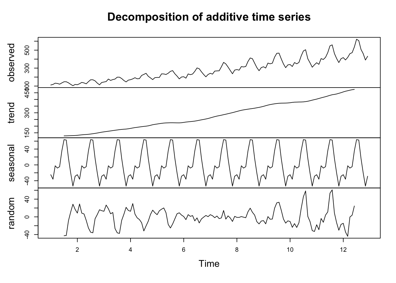
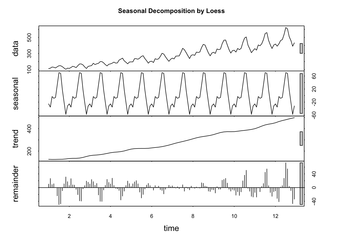
The result of the additive, classical decomposition analysis clearly shows that a positive trend is present. In addition, a strong seasonal component (showing a distinctive, regular pattern) is present which leads us to believe that it should be possible to generate predictions about the time series based on historical information.

A detailed look at the y-axes of the plots reveals that the trend component is much more important than seasonality.

146.1.3 Interpretation

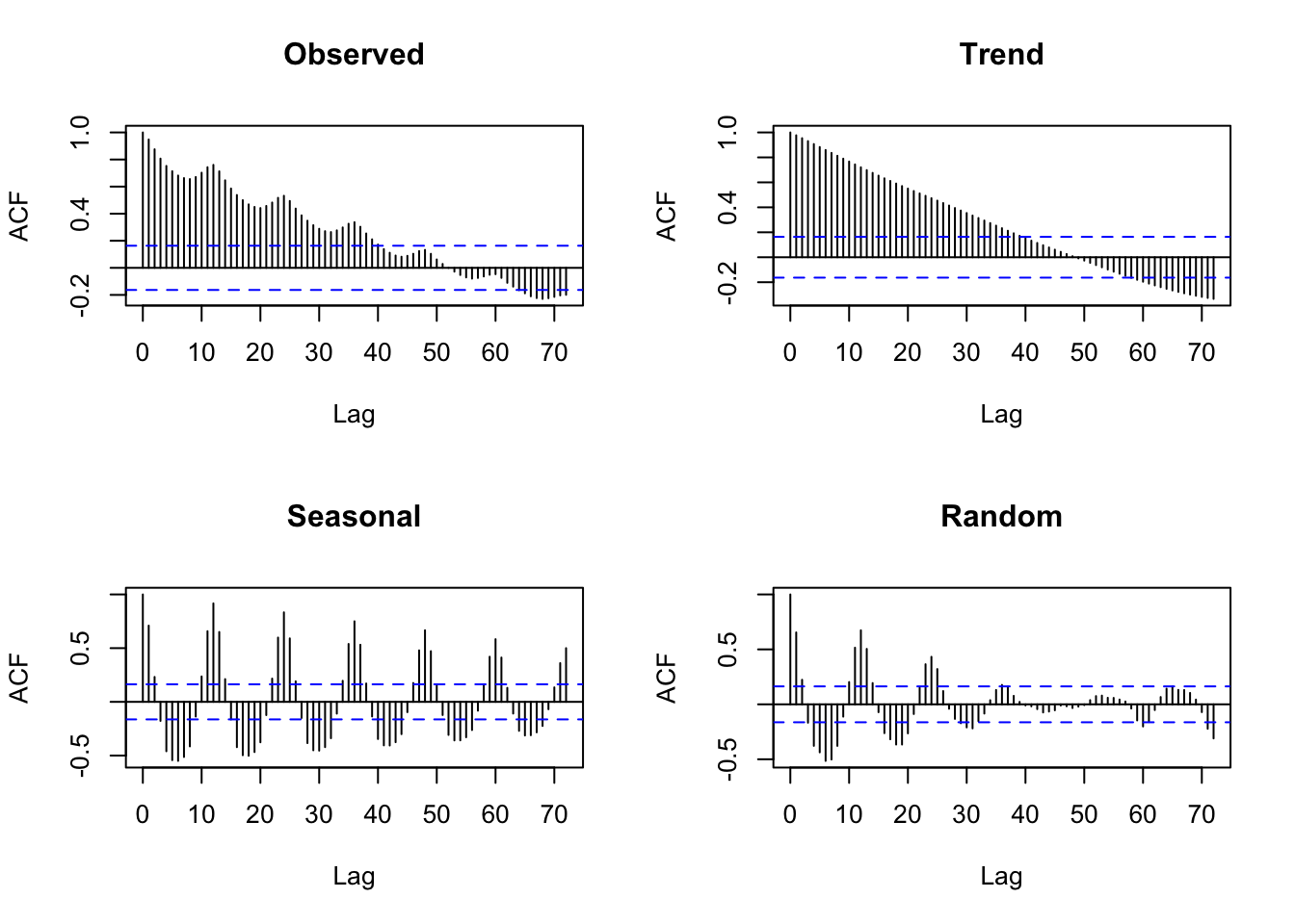
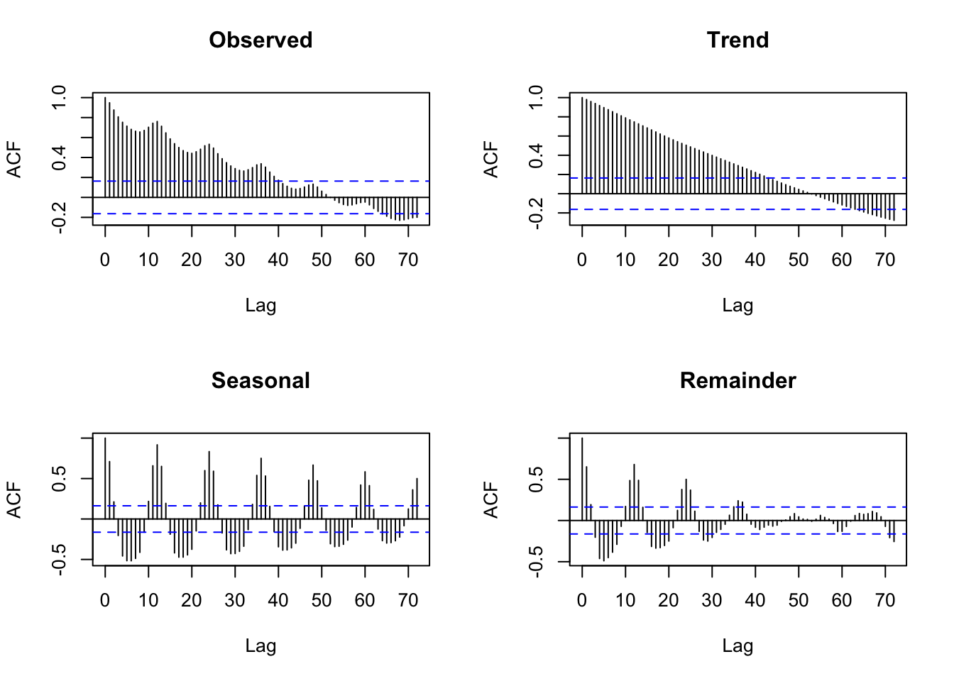
A much better way to identify the previously mentioned properties is to make use of the Autocorrelation Function (ACF). The ACF of the Classical Decomposition can be obtained by changing the setting in the Type of Plot selection list and shows some remarkable features. For background on interpreting these diagnostics, see the (P)ACF chapter (PACF.qmd) and the periodogram chapter (Chapter 93):

The trend component exhibits a slowly (linearly) decreasing series of autocorrelation coefficients. This is the typical pattern for a long-run trend¹.
The seasonal component shows persistent (non-decaying) positive autocorrelation spikes at time lags \(k = 12, 24, 36, \ldots\). This is the typical pattern of strong deterministic seasonality.
Finally, the error component² displayed in the Figure shows a (regular) series of non-zero autocorrelations (significant at the 5% type I error level). This is important because it implies that the prediction errors of the Classical Decomposition model are not independent (they are in fact autocorrelated). In other words: past prediction errors contain systematic information that can be used to predict future prediction errors - hence, they can also be used to improve the forecasts of the time series.

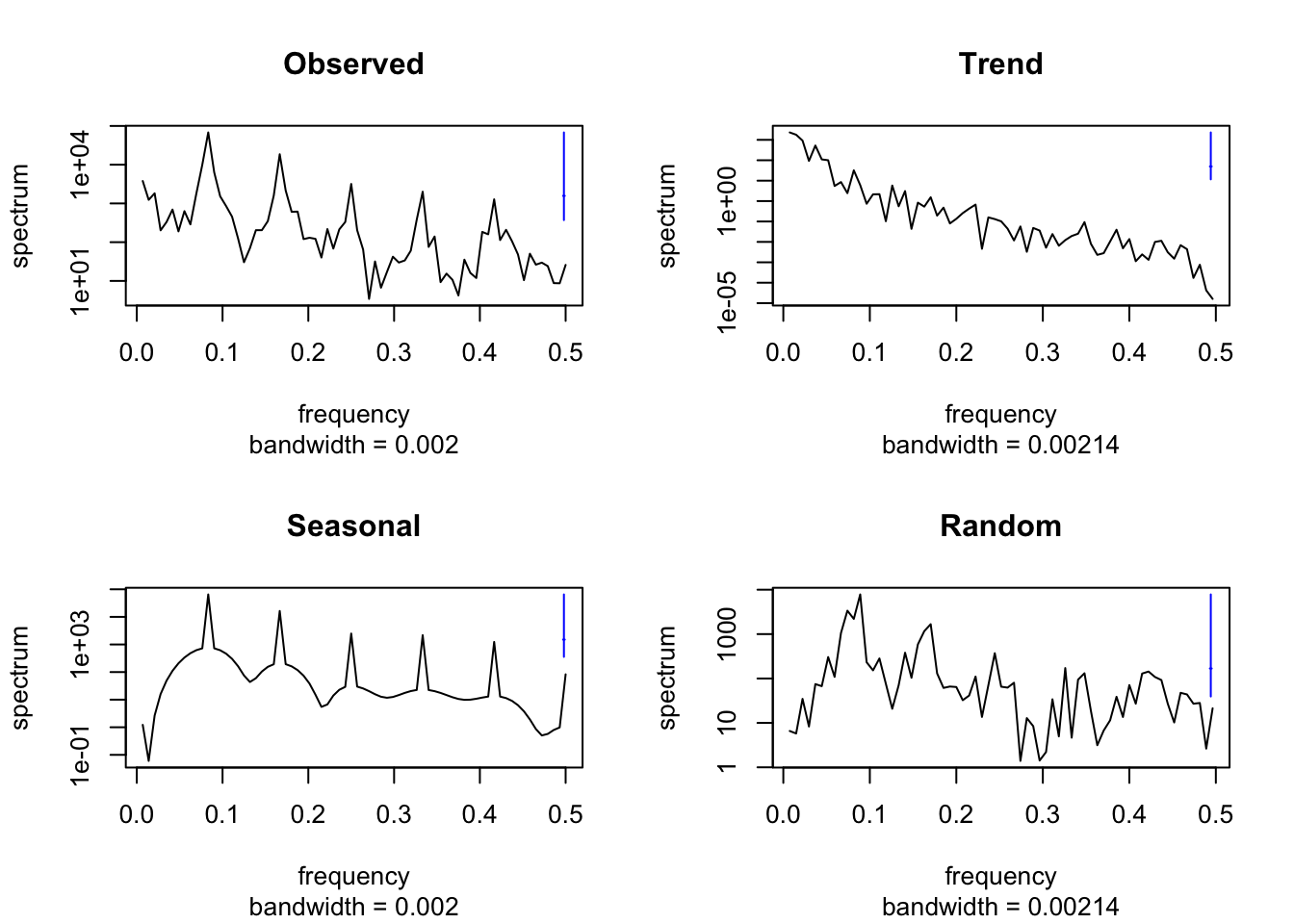
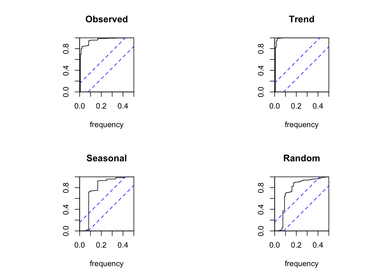
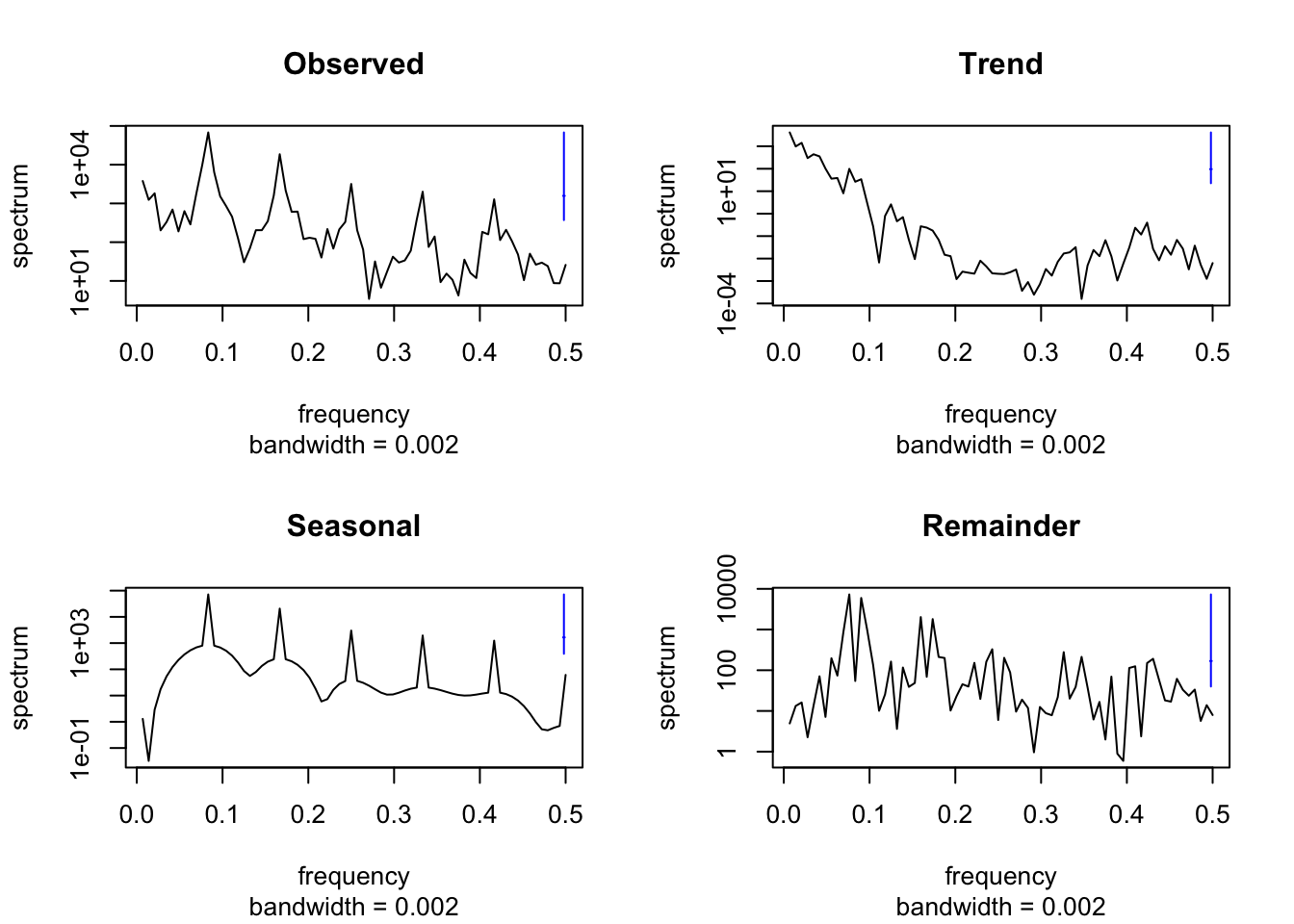
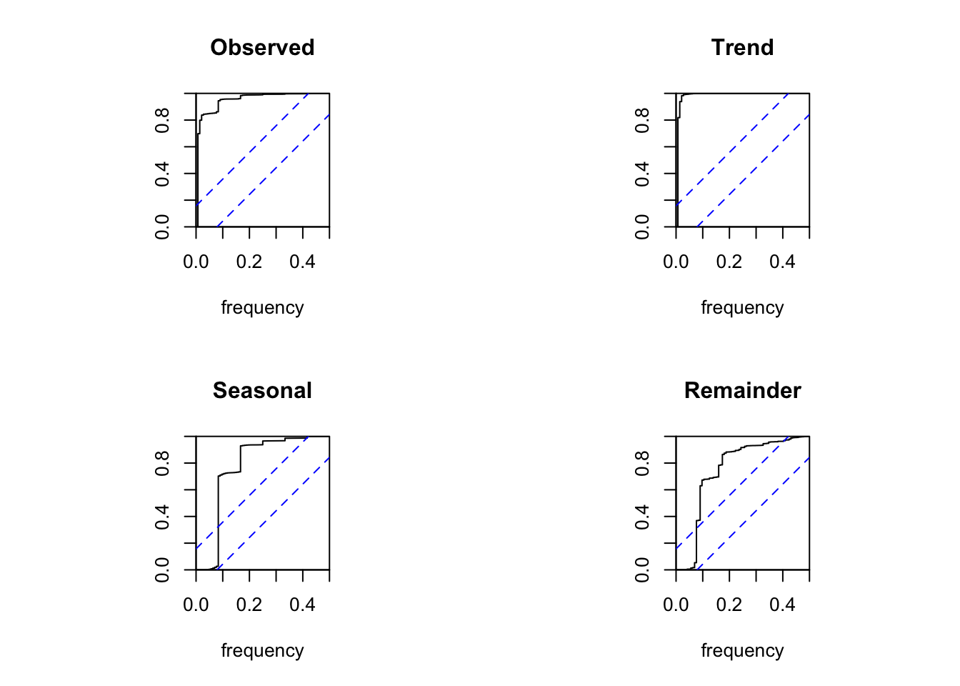
Of course, we can also compute the periodogram or cumulative periodogram to examine the components of the decomposition. The bottom line, however, is always the same and leads to identical conclusions.

146.1.4 Conclusion

There are two conclusions from this analysis:

A forecasting model that is based only on Moving Averages is incomplete and should be used with caution.
The model clearly indicates the presence of a long-run trend and a strongly seasonal pattern that can be predicted (but we need a more sophisticated model).

If you prefer to compute the Classical Decomposition on your local machine, the following script can be used in the R console:

Note: the local script below uses AirPassengers as a generic template dataset. The embedded app and chapter interpretation use the HPC series, so numeric outputs will differ unless you replace x with the HPC data.

x <- AirPassengers
par1 = 'additive' #Type of Seasonality 
par2 = 12 #Seasonal Period 
x <- ts(x, frequency = par2)
m <- decompose(x,type=par1)
plot(m)

mylagmax <- length(x)/2
op <- par(mfrow = c(2,2))
acf(as.numeric(x),lag.max = mylagmax,main='Observed')
acf(as.numeric(m$trend),na.action=na.pass,lag.max = mylagmax,main='Trend')
acf(as.numeric(m$seasonal),na.action=na.pass,lag.max = mylagmax,main='Seasonal')
acf(as.numeric(m$random),na.action=na.pass,lag.max = mylagmax,main='Random')

par(op)
op <- par(mfrow = c(2,2))
spectrum(as.numeric(x),main='Observed')
spectrum(as.numeric(m$trend[!is.na(m$trend)]),main='Trend')
spectrum(as.numeric(m$seasonal[!is.na(m$seasonal)]),main='Seasonal')
spectrum(as.numeric(m$random[!is.na(m$random)]),main='Random')

par(op)
op <- par(mfrow = c(2,2))
cpgram(as.numeric(x),main='Observed')
cpgram(as.numeric(m$trend[!is.na(m$trend)]),main='Trend')
cpgram(as.numeric(m$seasonal[!is.na(m$seasonal)]),main='Seasonal')
cpgram(as.numeric(m$random[!is.na(m$random)]),main='Random')

par(op)

146.1.5 Assignment

Compare the additive and multiplicative models:

Which model is better?
When would you (theoretically) expect a large difference between the additive and multiplicative model³
Apply additive and multiplicative decomposition to the Airline time series to empirically verify the theoretical answer⁴.

146.2 Seasonal Decomposition of Time Series by Loess

146.2.1 Model reference

Seasonal Decomposition by Loess is more sophisticated than the previous method and is described in full detail in Cleveland et al. (1990).

Interactive Shiny app (click to load).

Open in new tab

146.2.2 Analysis

The HPC time series was analyzed by the R module “Decomposition by Loess” which is available on-line:

https://shiny.wessa.net/decomposition/
RFC menu item Time Series / Decomposition

Based on the default parameters, the Decomposition by Loess analysis clearly confirms the positive long-run trend. Similarly, the seasonal component shows a distinctive, regular pattern just like in the previous model.

If you prefer to compute the Seasonal Loess Decomposition on your local machine, the following script can be used in the R console:

x <- AirPassengers
par1 = 12 #Seasonal period
par2 = 'periodic' #Seasonal window
par3 = 0 #Seasonal degree
par4 = NULL #Trend window
par5 = 1 #Trend degree
par6 = '' #Low-pass window
par7 = 1 #Low-pass degree
par8 = FALSE #Robust loess fitting
main = 'Seasonal Decomposition by Loess'
nx <- length(x)
x <- ts(x,frequency=par1)
if (par6 != '') {
  m <- stl(x,s.window=par2, s.degree=par3, t.window=par4, t.degree=par5, l.window=par6, l.degree=par7, robust=par8)
} else {
  m <- stl(x,s.window=par2, s.degree=par3, t.window=par4, t.degree=par5, l.degree=par7, robust=par8)
}
plot(m,main=main)

mylagmax <- nx/2
op <- par(mfrow = c(2,2))
acf(as.numeric(x),lag.max = mylagmax,main='Observed')
acf(as.numeric(m$time.series[,'trend']),na.action=na.pass,lag.max = mylagmax,main='Trend')
acf(as.numeric(m$time.series[,'seasonal']),na.action=na.pass,lag.max = mylagmax,main='Seasonal')
acf(as.numeric(m$time.series[,'remainder']),na.action=na.pass,lag.max = mylagmax,main='Remainder')

par(op)
op <- par(mfrow = c(2,2))
spectrum(as.numeric(x),main='Observed')
spectrum(as.numeric(m$time.series[!is.na(m$time.series[,'trend']),'trend']),main='Trend')
spectrum(as.numeric(m$time.series[!is.na(m$time.series[,'seasonal']),'seasonal']),main='Seasonal')
spectrum(as.numeric(m$time.series[!is.na(m$time.series[,'remainder']),'remainder']),main='Remainder')

par(op)
op <- par(mfrow = c(2,2))
cpgram(as.numeric(x),main='Observed')
cpgram(as.numeric(m$time.series[!is.na(m$time.series[,'trend']),'trend']),main='Trend')
cpgram(as.numeric(m$time.series[!is.na(m$time.series[,'seasonal']),'seasonal']),main='Seasonal')
cpgram(as.numeric(m$time.series[!is.na(m$time.series[,'remainder']),'remainder']),main='Remainder')

par(op)

146.2.3 Assignment

Compare the analysis of Classical Decomposition and Seasonal Decomposition by Loess. Answer the following questions for both methods:

Is the trend component more important than the seasonal?
Describe the typical pattern of the Autocorrelation Function for all components
Interpret and describe the autocorrelation plots in your own words
Is the second (that is, more sophisticated) method doing a better job⁵?

It does not matter if the trend is positive or negative - the ACF pattern is the same in both cases.↩︎
In the R module this is called the “random” term.↩︎
Hint: think about how the seasonal pattern may become stronger (on the long run) as the number of consumers in the HPC market grows. In other words, there may be a relationship between the long-run trend and the seasonal component. This question is also closely related to the concept of heteroskedasticity (for a formal treatment, see Chapter 143).↩︎
The Airline Passenger time series is - unlike the HPC time series - characterized by the fact that seasonality becomes stronger as the level of Airline passengers grows. There is a direct relationship between trend and seasonality which is a special case of heteroskedasticity.↩︎
Hint: the words “random” and “remainder” both relate to the prediction error (they are synonyms).↩︎