• Descriptive
    • Moments
    • Concentration
    • Central Tendency
    • Variability
    • Stem-and-Leaf Plot
    • Histogram & Frequency Table
    • Data Quality Forensics
    • Conditional EDA
    • Quantiles
    • Kernel Density Estimation
    • Normal QQ Plot
    • Bootstrap Plot

    • Multivariate Descriptive Statistics
  • Distributions
    • Binomial Probabilities
    • Geometric Probabilities
    • Negative Binomial Probabilities
    • Hypergeometric Probabilities
    • Multinomial Probabilities
    • Poisson Probabilities

    • Exponential
    • Gamma
    • Erlang
    • Weibull
    • Rayleigh
    • Lognormal
    • Pareto
    • Inverse Gamma

    • Beta
    • Power
    • Beta Prime (Inv. Beta)
    • Triangular

    • Normal (area)
    • Logistic
    • Laplace
    • Cauchy (standard)
    • Cauchy (location-scale)
    • Gumbel

    • Normal RNG
    • ML Fitting
    • Tukey Lambda PPCC
    • Box-Cox Normality Plot
    • Sample Correlation r

    • Empirical Tests
  • Hypotheses
    • Theoretical Aspects of Hypothesis Testing
    • Bayesian Inference
    • Minimum Sample Size

    • Empirical Tests
    • Multivariate (pair-wise) Testing
  • Models
    • Manual Model Building
  • Time Series
    • Time Series Plot
    • Decomposition
    • Exponential Smoothing

    • Blocked Bootstrap Plot
    • Mean Plot
    • (P)ACF
    • VRM
    • Standard Deviation-Mean Plot
    • Spectral Analysis
    • ARIMA

    • Cross Correlation Function
    • Granger Causality
  1. Probability Distributions
  2. 36  Logistic Distribution
  • Preface
  • Getting Started
    • 1  Introduction
    • 2  Why Do We Need Innovative Technology?
    • 3  Basic Definitions
    • 4  The Big Picture: Why We Analyze Data
  • Introduction to Probability
    • 5  Definitions of Probability
    • 6  Jeffreys’ axiom system
    • 7  Bayes’ Theorem
    • 8  Sensitivity and Specificity
    • 9  Naive Bayes Classifier
    • 10  Law of Large Numbers

    • 11  Problems
  • Probability Distributions
    • 12  Bernoulli Distribution
    • 13  Binomial Distribution
    • 14  Geometric Distribution
    • 15  Negative Binomial Distribution
    • 16  Hypergeometric Distribution
    • 17  Multinomial Distribution
    • 18  Poisson Distribution

    • 19  Uniform Distribution (Rectangular Distribution)
    • 20  Normal Distribution (Gaussian Distribution)
    • 21  Gaussian Naive Bayes Classifier
    • 22  Chi Distribution
    • 23  Chi-squared Distribution (1 parameter)
    • 24  Chi-squared Distribution (2 parameters)
    • 25  Student t-Distribution
    • 26  Fisher F-Distribution
    • 27  Exponential Distribution
    • 28  Lognormal Distribution
    • 29  Gamma Distribution
    • 30  Beta Distribution
    • 31  Weibull Distribution
    • 32  Pareto Distribution
    • 33  Inverse Gamma Distribution
    • 34  Rayleigh Distribution
    • 35  Erlang Distribution
    • 36  Logistic Distribution
    • 37  Laplace Distribution
    • 38  Gumbel Distribution
    • 39  Cauchy Distribution
    • 40  Triangular Distribution
    • 41  Power Distribution
    • 42  Beta Prime Distribution
    • 43  Sample Correlation Distribution

    • 44  Problems
  • Descriptive Statistics & Exploratory Data Analysis
    • 45  Types of Data
    • 46  Datasheets

    • 47  Frequency Plot (Bar Plot)
    • 48  Frequency Table
    • 49  Contingency Table
    • 50  Binomial Classification Metrics
    • 51  Confusion Matrix
    • 52  ROC Analysis

    • 53  Stem-and-Leaf Plot
    • 54  Histogram
    • 55  Data Quality Forensics
    • 56  Quantiles
    • 57  Central Tendency
    • 58  Variability
    • 59  Skewness & Kurtosis
    • 60  Concentration
    • 61  Notched Boxplot
    • 62  Scatterplot
    • 63  Pearson Correlation
    • 64  Rank Correlation
    • 65  Partial Pearson Correlation
    • 66  Simple Linear Regression
    • 67  Moments
    • 68  Quantile-Quantile Plot (QQ Plot)
    • 69  Normal Probability Plot
    • 70  Probability Plot Correlation Coefficient Plot (PPCC Plot)
    • 71  Box-Cox Normality Plot
    • 72  Kernel Density Estimation
    • 73  Bivariate Kernel Density Plot
    • 74  Conditional EDA: Panel Diagnostics
    • 75  Bootstrap Plot (Central Tendency)
    • 76  Survey Scores Rank Order Comparison
    • 77  Cronbach Alpha

    • 78  Equi-distant Time Series
    • 79  Time Series Plot (Run Sequence Plot)
    • 80  Mean Plot
    • 81  Blocked Bootstrap Plot (Central Tendency)
    • 82  Standard Deviation-Mean Plot
    • 83  Variance Reduction Matrix
    • 84  (Partial) Autocorrelation Function
    • 85  Periodogram & Cumulative Periodogram

    • 86  Problems
  • Hypothesis Testing
    • 87  Normal Distributions revisited
    • 88  The Population
    • 89  The Sample
    • 90  The One-Sided Hypothesis Test
    • 91  The Two-Sided Hypothesis Test
    • 92  When to use a one-sided or two-sided test?
    • 93  What if \(\sigma\) is unknown?
    • 94  The Central Limit Theorem (revisited)
    • 95  Statistical Test of the Population Mean with known Variance
    • 96  Statistical Test of the Population Mean with unknown Variance
    • 97  Statistical Test of the Variance
    • 98  Statistical Test of the Population Proportion
    • 99  Statistical Test of the Standard Deviation \(\sigma\)
    • 100  Statistical Test of the difference between Means -- Independent/Unpaired Samples
    • 101  Statistical Test of the difference between Means -- Dependent/Paired Samples
    • 102  Statistical Test of the difference between Variances -- Independent/Unpaired Samples

    • 103  Hypothesis Testing for Research Purposes
    • 104  Decision Thresholds, Alpha, and Confidence Levels
    • 105  Bayesian Inference for Decision-Making
    • 106  One Sample t-Test
    • 107  Skewness & Kurtosis Tests
    • 108  Paired Two Sample t-Test
    • 109  Wilcoxon Signed-Rank Test
    • 110  Unpaired Two Sample t-Test
    • 111  Unpaired Two Sample Welch Test
    • 112  Two One-Sided Tests (TOST) for Equivalence
    • 113  Mann-Whitney U test (Wilcoxon Rank-Sum Test)
    • 114  Bayesian Two Sample Test
    • 115  Median Test based on Notched Boxplots
    • 116  Chi-Squared Tests for Count Data
    • 117  Kolmogorov-Smirnov Test
    • 118  One Way Analysis of Variance (1-way ANOVA)
    • 119  Kruskal-Wallis Test
    • 120  Two Way Analysis of Variance (2-way ANOVA)
    • 121  Repeated Measures ANOVA
    • 122  Friedman Test
    • 123  Testing Correlations
    • 124  A Note on Causality

    • 125  Problems
  • Regression Models
    • 126  Simple Linear Regression Model (SLRM)
    • 127  Multiple Linear Regression Model (MLRM)
    • 128  Logistic Regression
    • 129  Generalized Linear Models
    • 130  Multinomial and Ordinal Logistic Regression
    • 131  Cox Proportional Hazards Regression
    • 132  Conditional Inference Trees
    • 133  Leaf Diagnostics for Conditional Inference Trees
    • 134  Hypothesis Testing with Linear Regression Models (from a Practical Point of View)

    • 135  Problems
  • Introduction to Time Series Analysis
    • 136  Case: the Market of Health and Personal Care Products
    • 137  Decomposition of Time Series
    • 138  Ad hoc Forecasting of Time Series
  • Box-Jenkins Analysis
    • 139  Introduction to Box-Jenkins Analysis
    • 140  Theoretical Concepts
    • 141  Stationarity
    • 142  Identifying ARMA parameters
    • 143  Estimating ARMA Parameters and Residual Diagnostics
    • 144  Forecasting with ARIMA models
    • 145  Intervention Analysis
    • 146  Cross-Correlation Function
    • 147  Transfer Function Noise Models
    • 148  General-to-Specific Modeling
  • References
  • Appendices
    • Appendices
    • A  Method Selection Guide
    • B  Presentations and Teaching Materials
    • C  R Language Concepts for Statistical Computing
    • D  Matrix Algebra
    • E  Standard Normal Table (Gaussian Table)
    • F  Critical values of Student’s \(t\) distribution with \(\nu\) degrees of freedom
    • G  Upper-tail critical values of the \(\chi^2\)-distribution with \(\nu\) degrees of freedom
    • H  Lower-tail critical values of the \(\chi^2\)-distribution with \(\nu\) degrees of freedom

Table of contents

  • 36.1 Probability Density Function
  • 36.2 Purpose
  • 36.3 Distribution Function
  • 36.4 Moment Generating Function
  • 36.5 1st Uncentered Moment
  • 36.6 2nd Uncentered Moment
  • 36.7 3rd Uncentered Moment
  • 36.8 4th Uncentered Moment
  • 36.9 2nd Centered Moment
  • 36.10 3rd Centered Moment
  • 36.11 4th Centered Moment
  • 36.12 Expected Value
  • 36.13 Variance
  • 36.14 Median
  • 36.15 Mode
  • 36.16 Coefficient of Skewness
  • 36.17 Coefficient of Kurtosis
  • 36.18 Parameter Estimation
  • 36.19 R Module
    • 36.19.1 RFC
    • 36.19.2 Direct app link
    • 36.19.3 R Code
  • 36.20 Example
  • 36.21 Random Number Generator
  • 36.22 Property 1: Sigmoid CDF
  • 36.23 Property 2: Self-Referential Density
  • 36.24 Property 3: Heavier Tails than Normal
  • 36.25 Related Distributions 1: Normal Distribution
DRAFT This draft is under development — DO NOT CITE OR SHARE.
  1. Probability Distributions
  2. 36  Logistic Distribution

36  Logistic Distribution

The Logistic distribution resembles the Normal in shape but has heavier tails. Its CDF — the sigmoid function — is one of the most important functions in statistics and machine learning, forming the mathematical foundation of logistic regression and neural network activations.

Formally, the random variate \(X\) defined for all of \(\mathbb{R}\), is said to have a Logistic Distribution (i.e. \(X \sim \text{Logistic}(\mu, s)\)) with location parameter \(\mu \in \mathbb{R}\) and scale parameter \(s > 0\). In R, the built-in functions are dlogis(x, location = mu, scale = s), plogis, qlogis, and rlogis.

36.1 Probability Density Function

\[ f(x) = \frac{e^{-(x-\mu)/s}}{s\,(1+e^{-(x-\mu)/s})^2} = \frac{F(x)\,[1-F(x)]}{s} \]

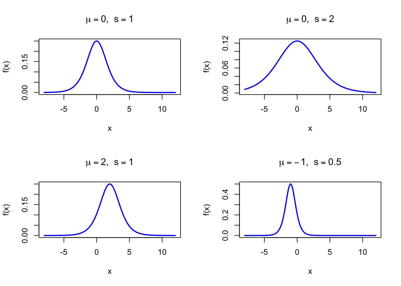
The figure below shows examples of the Logistic Probability Density Function for different parameter combinations.

Code
par(mfrow = c(2, 2))
x <- seq(-8, 12, length = 500)

plot(x, dlogis(x, location = 0, scale = 1), type = "l", lwd = 2, col = "blue",
     xlab = "x", ylab = "f(x)", main = expression(paste(mu == 0, ",  ", s == 1)))

plot(x, dlogis(x, location = 0, scale = 2), type = "l", lwd = 2, col = "blue",
     xlab = "x", ylab = "f(x)", main = expression(paste(mu == 0, ",  ", s == 2)))

plot(x, dlogis(x, location = 2, scale = 1), type = "l", lwd = 2, col = "blue",
     xlab = "x", ylab = "f(x)", main = expression(paste(mu == 2, ",  ", s == 1)))

plot(x, dlogis(x, location = -1, scale = 0.5), type = "l", lwd = 2, col = "blue",
     xlab = "x", ylab = "f(x)", main = expression(paste(mu == -1, ",  ", s == 0.5)))

par(mfrow = c(1, 1))
Figure 36.1: Logistic Probability Density Function for various parameter combinations

36.2 Purpose

The Logistic distribution is a symmetric, unimodal distribution on \(\mathbb{R}\) that closely resembles the Normal but has heavier tails. Its CDF — the logistic sigmoid function — plays a fundamental role in binary classification models. Common applications include:

  • Logistic regression: the latent continuous variable whose sign determines the binary outcome
  • Neural networks: the sigmoid activation function is the Logistic CDF
  • Growth curve modeling (logistic growth) in biology and ecology
  • Bioassay and dose-response modeling where response probability increases with dose
  • Heavy-tailed alternative to the Normal for symmetric continuous data

Relation to the discrete setting. The Logistic distribution is the continuous analog of the Binomial distribution via the logit link: the Binomial models discrete 0/1 outcomes, while the Logistic models their continuous log-odds representation. In logistic regression, binary Binomial outcomes are modeled with a Logistic-distributed latent variable.

36.3 Distribution Function

\[ F(x) = \frac{1}{1+e^{-(x-\mu)/s}} \]

This is the logistic sigmoid function, one of the most widely used functions in statistics and machine learning.

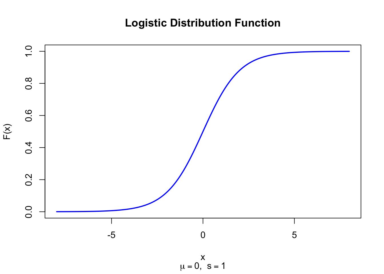
The figure below shows the Logistic Distribution Function for \(\mu = 0\) and \(s = 1\).

Code
x <- seq(-8, 8, length = 500)
plot(x, plogis(x, location = 0, scale = 1), type = "l", lwd = 2, col = "blue",
     xlab = "x", ylab = "F(x)", main = "Logistic Distribution Function",
     sub = expression(paste(mu == 0, ",  ", s == 1)))
Figure 36.2: Logistic Distribution Function (location = 0, scale = 1)

36.4 Moment Generating Function

\[ M_X(t) = e^{\mu t}\,\frac{\pi s t}{\sin(\pi s t)}, \quad |t| < \frac{1}{s} \]

36.5 1st Uncentered Moment

\[ \mu_1' = \mu \]

36.6 2nd Uncentered Moment

\[ \mu_2' = \mu^2 + \frac{s^2\pi^2}{3} \]

36.7 3rd Uncentered Moment

\[ \mu_3' = \mu^3 + \mu s^2\pi^2 \]

36.8 4th Uncentered Moment

\[ \mu_4' = \mu^4 + 2\mu^2 s^2\pi^2 + \frac{7s^4\pi^4}{15} \]

36.9 2nd Centered Moment

\[ \mu_2 = \frac{s^2\pi^2}{3} \]

36.10 3rd Centered Moment

\[ \mu_3 = 0 \]

The distribution is symmetric about \(\mu\), so all odd centered moments vanish.

36.11 4th Centered Moment

\[ \mu_4 = \frac{7s^4\pi^4}{15} \]

36.12 Expected Value

\[ \text{E}(X) = \mu \]

36.13 Variance

\[ \text{V}(X) = \frac{s^2\pi^2}{3} \]

36.14 Median

\[ \text{Med}(X) = \mu \]

36.15 Mode

\[ \text{Mo}(X) = \mu \]

36.16 Coefficient of Skewness

\[ g_1 = 0 \]

The distribution is symmetric about \(\mu\).

36.17 Coefficient of Kurtosis

\[ g_2 = \frac{\mu_4}{\mu_2^2} = \frac{7s^4\pi^4/15}{s^4\pi^4/9} = \frac{63}{15} = \frac{21}{5} = 4.2 \]

The excess kurtosis is \(g_2 - 3 = 1.2\), indicating heavier tails than the Normal distribution.

36.18 Parameter Estimation

Maximum likelihood estimates are obtained numerically in R:

library(MASS)

set.seed(42)
x_obs <- rlogis(100, location = 70, scale = 5)

fit <- fitdistr(x_obs, "logistic")
print(fit)
    location      scale   
  70.7404214    5.6983159 
 ( 0.9767560) ( 0.4816192)

36.19 R Module

36.19.1 RFC

The Logistic Distribution module is available in RFC under the menu “Distributions / Logistic Distribution”.

36.19.2 Direct app link

  • https://shiny.wessa.net/logistic/

36.19.3 R Code

The following code demonstrates Logistic probability calculations:

mu <- 70; s <- 5

# Probability density function
dlogis(60, location = mu, scale = s)

# Distribution function: P(X <= 60)
plogis(60, location = mu, scale = s)

# Quantile function (median)
qlogis(0.5, location = mu, scale = s)

# Generate random Logistic numbers
set.seed(42)
rlogis(10, location = mu, scale = s)

# Standard deviation
cat("SD:", s * pi / sqrt(3), "\n")
[1] 0.02099872
[1] 0.1192029
[1] 70
 [1] 81.86891 83.50413 65.42896 77.94401 72.91474 70.38210 75.14155 60.69844
 [9] 73.24960 74.35767
SD: 9.068997 

36.20 Example

Exam scores in a large class are modeled as \(X \sim \text{Logistic}(\mu = 70, s = 5)\). We compute the probability of scoring below 60.

mu <- 70; s <- 5

# P(score < 60)
cat("P(score < 60):", plogis(60, location = mu, scale = s), "\n")

# P(score > 80)
cat("P(score > 80):", 1 - plogis(80, location = mu, scale = s), "\n")

# Mean, median, SD
cat("Mean (= median):", mu, "\n")
cat("SD:", round(s * pi / sqrt(3), 4), "\n")
P(score < 60): 0.1192029 
P(score > 80): 0.1192029 
Mean (= median): 70 
SD: 9.069 
Interactive Shiny app (click to load).
Open in new tab

36.21 Random Number Generator

Logistic random variates are generated via the inverse-CDF method. Since \(F(x) = 1/(1+e^{-(x-\mu)/s})\), the quantile function is the log-odds (logit) function:

\[ X = \mu - s\ln\!\left(\frac{1}{U} - 1\right) \sim \text{Logistic}(\mu, s) \quad \text{when } U \sim \text{U}(0,1) \]

set.seed(123)
n <- 1000; mu <- 0; s <- 1

# Inverse-transform method
u <- runif(n)
x_inv <- mu - s * log(1/u - 1)

# Compare with rlogis
x_rlogis <- rlogis(n, location = mu, scale = s)

cat("Inverse-transform: mean =", round(mean(x_inv), 4),
    "  var =", round(var(x_inv), 4), "\n")
cat("rlogis():          mean =", round(mean(x_rlogis), 4),
    "  var =", round(var(x_rlogis), 4), "\n")
cat("Theoretical:       mean =", mu,
    "  var =", round(s^2 * pi^2 / 3, 4), "\n")
Inverse-transform: mean = -0.0202   var = 3.2444 
rlogis():          mean = -0.0087   var = 3.2559 
Theoretical:       mean = 0   var = 3.2899 
Interactive Shiny app (click to load).
Open in new tab

36.22 Property 1: Sigmoid CDF

The CDF \(F(x) = 1/(1+e^{-(x-\mu)/s})\) is the logistic sigmoid function — the foundation of logistic regression. The log-odds (logit) of \(F(x)\) is linear in \(x\):

\[ \text{logit}(F(x)) = \ln\!\frac{F(x)}{1-F(x)} = \frac{x - \mu}{s} \]

36.23 Property 2: Self-Referential Density

The density can be expressed in terms of the CDF:

\[ f(x) = \frac{F(x)\,[1-F(x)]}{s} \]

This elegant identity is unique to the Logistic distribution and is exploited in the derivation of the logistic regression score equations.

36.24 Property 3: Heavier Tails than Normal

The Logistic distribution has kurtosis \(g_2 = 4.2\) versus \(g_2 = 3\) for the Normal. This means the Logistic assigns more probability to values far from the mean — a feature that makes it more robust to outliers in some applications.

36.25 Related Distributions 1: Normal Distribution

The Normal distribution has the same symmetric, bell-shaped form but lighter tails (\(g_2 = 3\)). For most practical purposes, the two distributions are very similar near the center but differ in the tails (see Chapter 20).

35  Erlang Distribution
37  Laplace Distribution

© 2026 Patrick Wessa. Provided as-is, without warranty.

Feedback: e-mail | Anonymous contributions: click to copy (Sats) | click to copy (XMR)

Cookie Preferences