DRAFT This draft is under development — DO NOT CITE OR SHARE.

148  General-to-Specific Modeling

The Box-Jenkins methodology follows an iterative cycle of identification, estimation, and diagnostics. This chapter places that methodology in the broader context of general-to-specific (GtS) modeling, formalised by David Hendry (Hendry 1995) and the London School of Economics econometrics tradition. We also introduce error correction models (ECMs) for cointegrated series following Engle and Granger (Engle and Granger 1987), with links to Johansen-type system approaches (Johansen 1988).

148.1 The Hendry Methodology

The general-to-specific approach starts with a deliberately over-parameterized model — one that includes more variables and lags than are likely needed — and systematically simplifies it. The final “specific” model must satisfy three conditions:

1. It is parsimonious and interpretable (no unnecessary terms)
2. Residuals pass diagnostic tests (no autocorrelation, normality, constant variance)
3. The model encompasses rival specifications (it can explain what competitors explain, but not vice versa)

This stands in contrast to the “specific-to-general” approach, where one starts with a simple model and adds complexity. The GtS philosophy argues that starting general avoids the risk of omitted variable bias and that the data — not the analyst’s prior beliefs — should determine which variables survive.

148.1.1 Connection to Box-Jenkins

The ARIMA backward selection procedure in Chapter 143 is already GtS in spirit: we start with maximum values for \(p\), \(q\), \(P\), and \(Q\), estimate all parameters, and simplify step by step. Hendry formalised and extended this principle to include:

• Exogenous variables (regressors beyond the series’ own lags)
• Error correction terms (for cointegrated series, see Section 148.3)
• Structural breaks (intervention variables, as in Chapter 145)
• Congruence checks (a battery of diagnostic tests applied at each step)

The ARIMA backward selection and the GtS dynamic regression are two implementations of the same underlying principle: let a general model simplify itself under the discipline of statistical testing and diagnostic checking.

148.2 Worked Example: Dynamic Regression with Coffee Prices

We demonstrate the GtS approach using the Coffee dataset (the same data from Section 146.4 and Section 147.5). We model the US retail price (\(Y\)) as a function of its own lags and lagged values of the Colombian import price (\(X\)).

Interactive Shiny app (click to load).

Open in new tab

148.2.1 Step 1: The General Model

Start with an over-parameterized dynamic regression:

\[ Y_t = \alpha + \sum_{i=1}^{6} \beta_i Y_{t-i} + \sum_{j=0}^{6} \gamma_j X_{t-j} + e_t \]

This includes 6 lags of \(Y\) and the contemporaneous plus 6 lagged values of \(X\) — 14 parameters in total (including the intercept).

coffee <- read.csv("coffee.csv")
colombia <- coffee$Colombia
usa <- coffee$USA
n <- length(usa)

# Create a data frame with lagged variables
max_lag <- 6
start_idx <- max_lag + 1

df <- data.frame(y = usa[start_idx:n])
for (i in 1:max_lag) {
  df[[paste0("y_lag", i)]] <- usa[(start_idx - i):(n - i)]
}
for (j in 0:max_lag) {
  df[[paste0("x_lag", j)]] <- colombia[(start_idx - j):(n - j)]
}

# Fit the general model
fit_general <- lm(y ~ ., data = df)
cat("General model (14 parameters):\n")
print(summary(fit_general))

General model (14 parameters):

Call:
lm(formula = y ~ ., data = df)

Residuals:
    Min      1Q  Median      3Q     Max 
-32.597  -4.350  -0.683   2.984  78.881 

Coefficients:
            Estimate Std. Error t value Pr(>|t|)    
(Intercept) 11.37662    3.63923   3.126  0.00192 ** 
y_lag1       1.28555    0.05443  23.620  < 2e-16 ***
y_lag2      -0.49078    0.08858  -5.540 6.06e-08 ***
y_lag3       0.21954    0.09233   2.378  0.01797 *  
y_lag4      -0.12906    0.09228  -1.399  0.16286    
y_lag5       0.03819    0.08842   0.432  0.66606    
y_lag6       0.01606    0.05109   0.314  0.75351    
x_lag0       0.31326    0.10360   3.024  0.00269 ** 
x_lag1       0.01003    0.15061   0.067  0.94695    
x_lag2      -0.04182    0.15047  -0.278  0.78121    
x_lag3      -0.01181    0.14797  -0.080  0.93641    
x_lag4       0.05620    0.15067   0.373  0.70939    
x_lag5       0.08837    0.15078   0.586  0.55819    
x_lag6      -0.32248    0.10766  -2.996  0.00294 ** 
---
Signif. codes:  0 '***' 0.001 '**' 0.01 '*' 0.05 '.' 0.1 ' ' 1

Residual standard error: 9.777 on 340 degrees of freedom
Multiple R-squared:  0.9616,    Adjusted R-squared:  0.9601 
F-statistic: 654.9 on 13 and 340 DF,  p-value: < 2.2e-16

148.2.2 Step 2: Simplify

In this chapter we use AIC-based backward elimination (step()), not p-value pruning. Mechanically, step() starts from the full model, tries dropping one term at a time, keeps the drop that gives the largest AIC improvement, and repeats until no further drop improves AIC.

# Backward elimination by AIC (set trace = 1 to show each elimination step)
fit_specific <- step(fit_general, direction = "backward", trace = 0)
cat("Specific model after backward elimination:\n")
print(summary(fit_specific))

Specific model after backward elimination:

Call:
lm(formula = y ~ y_lag1 + y_lag2 + y_lag3 + x_lag0 + x_lag6, 
    data = df)

Residuals:
    Min      1Q  Median      3Q     Max 
-33.590  -4.410  -0.531   2.737  81.223 

Coefficients:
            Estimate Std. Error t value Pr(>|t|)    
(Intercept) 11.43958    3.37382   3.391 0.000777 ***
y_lag1       1.27942    0.05356  23.886  < 2e-16 ***
y_lag2      -0.45549    0.08317  -5.477 8.31e-08 ***
y_lag3       0.11658    0.05227   2.230 0.026367 *  
x_lag0       0.31376    0.04777   6.568 1.86e-10 ***
x_lag6      -0.22693    0.04951  -4.583 6.39e-06 ***
---
Signif. codes:  0 '***' 0.001 '**' 0.01 '*' 0.05 '.' 0.1 ' ' 1

Residual standard error: 9.719 on 348 degrees of freedom
Multiple R-squared:  0.9612,    Adjusted R-squared:  0.9606 
F-statistic:  1722 on 5 and 348 DF,  p-value: < 2.2e-16

Recall that AIC (Akaike 1974) is defined (up to constants) as \(-2\\log L + 2k\), where \(k\) is the number of estimated parameters. Lower AIC indicates a better fit-complexity trade-off.

148.2.3 Step 3: Diagnostics

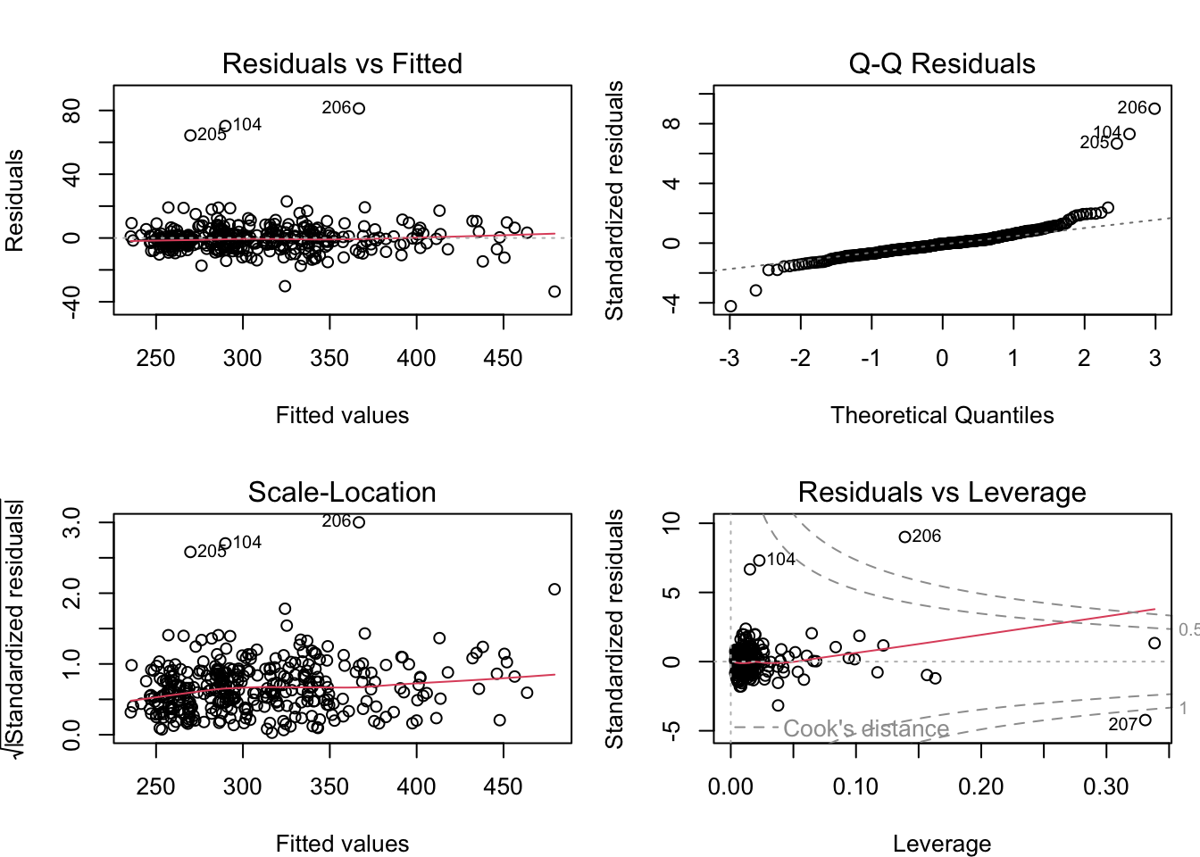
par(mfrow = c(2, 2), mar = c(4, 4, 3, 1))
plot(fit_specific)
par(mfrow = c(1, 1))

Figure 148.1: Residual diagnostics for the GtS dynamic regression

# Check residual autocorrelation
resid_gts <- residuals(fit_specific)
cat("Ljung-Box test on residuals:\n")
print(Box.test(resid_gts, lag = 24, type = "Ljung-Box"))

Ljung-Box test on residuals:

    Box-Ljung test

data:  resid_gts
X-squared = 13.055, df = 24, p-value = 0.9652

148.2.4 Comparison with the Transfer Function Model

# Compare AIC/BIC
cat("GtS dynamic regression AIC:", AIC(fit_specific), "\n")
cat("GtS dynamic regression BIC:", BIC(fit_specific), "\n")
cat("\nNumber of parameters in specific model:",
    length(coef(fit_specific)), "\n")

GtS dynamic regression AIC: 2622.612 
GtS dynamic regression BIC: 2649.697 

Number of parameters in specific model: 6 

The GtS dynamic regression and the transfer function model from Section 147.5 answer the same question — how does Colombia influence USA? — but use different parameterisations. The TF-noise model uses the \((r, s, b)\) structure identified from the CCF, while the GtS approach lets backward elimination determine which lags matter.

# Side-by-side out-of-sample comparison on the last 24 months
h <- 24
train_end <- n - h

# ---------- GtS one-step-ahead conditional predictions ----------
max_lag <- 6
start_idx <- max_lag + 1
df_all <- data.frame(y = usa[start_idx:n])
for (i in 1:max_lag) {
  df_all[[paste0("y_lag", i)]] <- usa[(start_idx - i):(n - i)]
}
for (j in 0:max_lag) {
  df_all[[paste0("x_lag", j)]] <- colombia[(start_idx - j):(n - j)]
}

train_rows <- 1:(train_end - max_lag)
test_rows <- (train_end - max_lag + 1):(n - max_lag)

fit_general_oos <- lm(y ~ ., data = df_all[train_rows, ])
fit_specific_oos <- step(fit_general_oos, direction = "backward", trace = 0)
pred_gts <- predict(fit_specific_oos, newdata = df_all[test_rows, ])
actual <- usa[(train_end + 1):n]

# ---------- Transfer function forecast ----------
xreg_lagged <- cbind(
  col_lag0 = as.numeric(colombia),
  col_lag1 = c(NA, as.numeric(colombia[-n])),
  col_lag2 = c(NA, NA, as.numeric(colombia[-c(n-1, n)])),
  col_lag3 = c(NA, NA, NA, as.numeric(colombia[-c(n-2, n-1, n)])),
  col_lag4 = c(NA, NA, NA, NA, as.numeric(colombia[-c(n-3, n-2, n-1, n)]))
)
tf_start <- 5
fit_tf_oos <- arima(usa[tf_start:train_end],
                    order = c(3, 1, 0),
                    xreg = xreg_lagged[tf_start:train_end, ])
fc_tf <- predict(fit_tf_oos, n.ahead = h,
                 newxreg = xreg_lagged[(train_end + 1):n, ])
pred_tf <- as.numeric(fc_tf$pred)

mae <- function(a, p) mean(abs(a - p), na.rm = TRUE)
rmse <- function(a, p) sqrt(mean((a - p)^2, na.rm = TRUE))

cmp <- data.frame(
  Model = c("GtS dynamic regression", "Transfer function (ARIMA+lagged xreg)"),
  MAE = c(mae(actual, pred_gts), mae(actual, pred_tf)),
  RMSE = c(rmse(actual, pred_gts), rmse(actual, pred_tf))
)
cat("Holdout comparison (last", h, "months):\n")
print(cmp, row.names = FALSE)

Holdout comparison (last 24 months):
                                 Model       MAE     RMSE
                GtS dynamic regression  9.552674 12.64849
 Transfer function (ARIMA+lagged xreg) 14.127852 18.29570

The table compares two non-identical forecasting setups on the same holdout. The GtS model uses one-step-ahead conditional predictions from selected lag regressors; the TF model uses multi-step ARIMA forecasts with lagged external inputs. The purpose is pedagogical: both approaches can be compared transparently on a common target series.

148.3 Error Correction Models (ECM)

148.3.1 Cointegration

When two time series \(X\) and \(Y\) are both non-stationary and integrated of the same order (typically \(I(1)\)), but an estimated linear combination \(Y_t - \\hat{\\beta} X_t\) is stationary (\(I(0)\)), the series are said to be cointegrated. Cointegration implies a long-run equilibrium relationship: the series may wander individually, but they do not drift apart without bound.

For the Coffee prices, cointegration would mean that Colombian import prices and US retail prices share a common long-run trend — which is economically plausible, as they reflect the same underlying commodity.

148.3.2 The Error Correction Model

If \(X\) and \(Y\) are cointegrated, the appropriate model is the Error Correction Model:

\[ \\Delta Y_t = \\text{short-run dynamics} + \\lambda_{ec} (Y_{t-1} - \\beta X_{t-1}) + e_t \]

The term \((Y_{t-1} - \\beta X_{t-1})\) is the error correction term: it measures how far the system is from its long-run equilibrium. The coefficient \(\\lambda_{ec}\) (typically negative) controls the speed of adjustment back to equilibrium.

148.3.3 Engle-Granger Two-Step Procedure

The Engle-Granger procedure tests for cointegration and estimates the ECM:

Step 1: Estimate the long-run relationship \(Y_t = \beta_0 + \beta_1 X_t + u_t\) by OLS.

Step 2: Test the residuals \(\hat{u}_t\) for stationarity using an augmented Dickey-Fuller (ADF) regression (Dickey and Fuller 1979) (with lagged differences). If the residuals are stationary, the series are cointegrated.

Step 3: If cointegrated, estimate the ECM using the lagged residuals as the error correction term.

library(lmtest)
library(urca)

coffee <- read.csv("coffee.csv")
colombia <- ts(coffee$Colombia, frequency = 12)
usa <- ts(coffee$USA, frequency = 12)

# Step 1: Long-run relationship
fit_lr <- lm(usa ~ colombia)
cat("Long-run relationship:\n")
cat("  USA =", round(coef(fit_lr)[1], 2), "+",
    round(coef(fit_lr)[2], 2), "* Colombia\n\n")

# Step 2: Test residuals for stationarity (ADF test)
resid_lr <- residuals(fit_lr)

# Residual-based ADF with lag augmentation (lag length selected by AIC)
eg_adf <- ur.df(resid_lr, type = "none", lags = 12, selectlags = "AIC")
cat("Residual-based ADF (Engle-Granger step 2):\n")
print(summary(eg_adf))

# Optional robustness cross-check: Phillips-Ouliaris cointegration test
po_test <- ca.po(cbind(usa, colombia), demean = "constant", type = "Pu")
cat("\nPhillips-Ouliaris cointegration test:\n")
print(summary(po_test))

# Step 3: ECM estimation (if cointegrated)
dy <- diff(as.numeric(usa))
dx <- diff(as.numeric(colombia))
ect_lag <- resid_lr[-length(resid_lr)]  # lagged equilibrium error

fit_ecm <- lm(dy ~ dx + ect_lag)
cat("Error Correction Model:\n")
print(summary(fit_ecm))

Long-run relationship:
  USA = 165.55 + 1.84 * Colombia

Residual-based ADF (Engle-Granger step 2):

############################################### 
# Augmented Dickey-Fuller Test Unit Root Test # 
############################################### 

Test regression none 


Call:
lm(formula = z.diff ~ z.lag.1 - 1 + z.diff.lag)

Residuals:
    Min      1Q  Median      3Q     Max 
-61.114  -5.955  -1.766   4.385  66.058 

Coefficients:
            Estimate Std. Error t value Pr(>|t|)   
z.lag.1     -0.07616    0.02346  -3.247  0.00128 **
z.diff.lag1  0.16321    0.05454   2.993  0.00297 **
z.diff.lag2 -0.10504    0.05413  -1.940  0.05315 . 
z.diff.lag3  0.10396    0.05433   1.914  0.05649 . 
z.diff.lag4 -0.13564    0.05378  -2.522  0.01212 * 
z.diff.lag5 -0.09799    0.05406  -1.813  0.07078 . 
---
Signif. codes:  0 '***' 0.001 '**' 0.01 '*' 0.05 '.' 0.1 ' ' 1

Residual standard error: 13.3 on 341 degrees of freedom
Multiple R-squared:  0.1094,    Adjusted R-squared:  0.09369 
F-statistic: 6.978 on 6 and 341 DF,  p-value: 5.165e-07


Value of test-statistic is: -3.2471 

Critical values for test statistics: 
      1pct  5pct 10pct
tau1 -2.58 -1.95 -1.62


Phillips-Ouliaris cointegration test:

######################################## 
# Phillips and Ouliaris Unit Root Test # 
######################################## 

Test of type Pu 
detrending of series with constant only 


Call:
lm(formula = z[, 1] ~ z[, -1])

Residuals:
    Min      1Q  Median      3Q     Max 
-104.10  -23.01   -1.58   28.30  106.62 

Coefficients:
             Estimate Std. Error t value Pr(>|t|)    
(Intercept) 165.55010    7.74054   21.39   <2e-16 ***
z[, -1]       1.84168    0.09701   18.98   <2e-16 ***
---
Signif. codes:  0 '***' 0.001 '**' 0.01 '*' 0.05 '.' 0.1 ' ' 1

Residual standard error: 34.65 on 358 degrees of freedom
Multiple R-squared:  0.5017,    Adjusted R-squared:  0.5003 
F-statistic: 360.4 on 1 and 358 DF,  p-value: < 2.2e-16


Value of test-statistic is: 66.5564 

Critical values of Pu are:
                  10pct   5pct    1pct
critical values 27.8536 33.713 48.0021

Error Correction Model:

Call:
lm(formula = dy ~ dx + ect_lag)

Residuals:
    Min      1Q  Median      3Q     Max 
-18.890  -5.370  -1.906   2.351 108.912 

Coefficients:
            Estimate Std. Error t value Pr(>|t|)    
(Intercept)  0.15140    0.59816   0.253 0.800330    
dx           0.37066    0.11025   3.362 0.000858 ***
ect_lag     -0.08426    0.01732  -4.864 1.73e-06 ***
---
Signif. codes:  0 '***' 0.001 '**' 0.01 '*' 0.05 '.' 0.1 ' ' 1

Residual standard error: 11.33 on 356 degrees of freedom
Multiple R-squared:  0.08827,   Adjusted R-squared:  0.08314 
F-statistic: 17.23 on 2 and 356 DF,  p-value: 7.188e-08

For the residual-based unit-root step, use the reported ADF critical values (or p-values), not standard \(t\)-test cutoffs. If the residual null of a unit root is rejected, cointegration is supported and the ECM is appropriate. The code above also computes the Phillips-Ouliaris (Phillips and Ouliaris 1990) residual-based cointegration test as an independent cross-check.

The coefficient of the error-correction term (\(\\hat{\\lambda}_{ec}\)) indicates adjustment speed. For example, \(\\hat{\\lambda}_{ec}=-0.10\) means roughly 10% of disequilibrium is corrected per period, while \(\\hat{\\lambda}_{ec}=-0.40\) indicates substantially faster adjustment. A significant negative coefficient is the expected sign in a stable ECM.

148.4 The Family Tree of Dynamic Models

The models covered in this part of the handbook form a coherent family, all sharing the Box-Jenkins foundation of separating systematic dynamics from noise and testing residuals for white noise.

Box-Jenkins (1970)
├── Univariate ARIMA
│   ├── Identification (ACF/PACF) ──── Ch. @sec-identifying-arma-parameters
│   ├── Estimation (backward sel.) ─── Ch. @sec-estimating-arma-parameters-and-residual-diagnostics
│   └── Forecasting ────────────────── Ch. @sec-forecasting-with-arima-models
│
├── Intervention Analysis ──────────── Ch. @sec-intervention-analysis
│   └── Binary inputs (pulse, step)
│
└── Transfer Function Noise ────────── Ch. @sec-transfer-function-noise
    └── Continuous inputs with lags
        │
        ├── Special case: ARIMAX (no lag dynamics)
        │
        └── Extensions:
            ├── Dynamic Regression / GtS ── This chapter
            ├── ECM / VECM (Engle-Granger, 1987; Johansen, 1988)
            ├── VAR (Sims, 1980) ── multiple equations
            ├── State-space (Harvey, Kalman) ── time-varying parameters
            └── Auto-ARIMA (Hyndman) ── automated identification

All of these models share a common diagnostic principle: if the residuals are not white noise, the model is missing something. The differences lie in how the systematic component is specified.

Note

The tsplot app (shiny.wessa.net/tsplot/) offers Prophet forecasts alongside ARIMA — a fundamentally different paradigm based on additive decomposition (trend + seasonality + holidays) rather than the stochastic difference equations of Box-Jenkins. The two paradigms answer the same forecasting question but make very different assumptions about the data-generating process.

148.5 What This Handbook Does Not (Yet) Cover

The models presented in this handbook cover the core Box-Jenkins framework and its most important extensions. Several natural follow-up topics are left for future editions:

• VAR / VECM: Vector autoregressive models for systems of multiple time series, where each series depends on its own lags and the lags of all other series (Sims 1980)
• State-space / structural time series models: Models where the parameters (trend, seasonal) are allowed to evolve over time (Harvey 1989)
• GARCH / volatility models: Models for time-varying variance (Engle 1982; Bollerslev 1986) — important in finance
• Machine learning approaches: Neural networks, gradient boosting, and other non-parametric methods applied to time series forecasting

These are all active areas of research and practice, and they build naturally on the foundation laid in this handbook.

148.6 Tasks

1. Apply the GtS approach to the Unemployment series with the financial crisis step dummy (from Section 145.6). Start with 6 AR lags and the step variable, then simplify. Compare the resulting model with the intervention ARIMA from Section 145.6.

2. Test for cointegration between Colombian and US coffee prices using the Engle-Granger procedure. If the series are cointegrated, estimate an ECM and interpret the speed of adjustment parameter.

3. Compare forecast accuracy for the last 24 months of USA retail coffee prices using four models: (a) pure ARIMA, (b) ARIMAX, (c) transfer function with lags, and (d) GtS dynamic regression. Which performs best on MAE and RMSE? Why might the results differ?

Akaike, Hirotugu. 1974. “A New Look at the Statistical Model Identification.” IEEE Transactions on Automatic Control 19 (6): 716–23. https://doi.org/10.1109/TAC.1974.1100705.

Bollerslev, Tim. 1986. “Generalized Autoregressive Conditional Heteroskedasticity.” Journal of Econometrics 31 (3): 307–27. https://doi.org/10.1016/0304-4076(86)90063-1.

Dickey, David A., and Wayne A. Fuller. 1979. “Distribution of the Estimators for Autoregressive Time Series with a Unit Root.” Journal of the American Statistical Association 74 (366): 427–31. https://doi.org/10.1080/01621459.1979.10482531.

Engle, Robert F. 1982. “Autoregressive Conditional Heteroscedasticity with Estimates of the Variance of United Kingdom Inflation.” Econometrica 50 (4): 987–1007. https://doi.org/10.2307/1912773.

Engle, Robert F., and Clive W. J. Granger. 1987. “Co-Integration and Error Correction: Representation, Estimation, and Testing.” Econometrica 55 (2): 251–76. https://doi.org/10.2307/1913236.

Harvey, Andrew C. 1989. Forecasting, Structural Time Series Models and the Kalman Filter. Cambridge: Cambridge University Press. https://doi.org/10.1017/CBO9781107049994.

Hendry, David F. 1995. Dynamic Econometrics. Oxford: Oxford University Press.

Johansen, Søren. 1988. “Statistical Analysis of Cointegration Vectors.” Journal of Economic Dynamics and Control 12 (2–3): 231–54. https://doi.org/10.1016/0165-1889(88)90041-3.

Phillips, Peter C. B., and Sam Ouliaris. 1990. “Asymptotic Properties of Residual Based Tests for Cointegration.” Econometrica 58 (1): 165–93. https://doi.org/10.2307/2938339.

Sims, Christopher A. 1980. “Macroeconomics and Reality.” Econometrica 48 (1): 1–48. https://doi.org/10.2307/1912017.