122 Bayesian Two Sample Test

122.1 Hypotheses

The Hypotheses are the same as for the ordinary Unpaired/Paired Two Sample t-Test. There is, however, a subtle difference in the way how “prior information” is treated. In traditional methods one can formulate two-sided Hypothesis Tests (without prior knowledge) or one-sided tests when there is “deterministic, prior information” about the sign of the difference of means.

Suppose an expert possesses prior knowledge which is probabilistic, rather than deterministic and that we are able to elicit the prior distributions (about the parameters in the Hypothesis Test) from the expert. In this scenario the prior distribution can be combined with the information from the data to obtain the so-called a posteriori distribution (much like the process which was used in the example in Chapter 7. The application of Bayes’ Theorem in Hypothesis Testing is called Bayesian Inference and (sometimes) requires the use of simulation or sampling methods (as is the case in the implementation of the Bayesian Two Sample Test in this section (Kruschke 2013)). For the general decision-threshold framing in Bayesian terms (posterior probabilities, Bayes factors, and decision risk), see Chapter 113.

122.2 Analysis based on posterior distribution

122.2.1 Software

The Bayesian Two Sample Test can be found on the public website: https://compute.wessa.net/rwasp_Bayesian_Two_Sample_Test.wasp.

122.2.2 Data & Parameters

This R module contains the following fields:

Data X: a multivariate dataset containing quantitative data
Names of X columns: a space delimited list of names (one name for each column)
Column number of first sample: a positive integer value of the column in the multivariate dataset which corresponds to the first sample
Column number of second sample: a positive integer value of the column in the multivariate dataset which corresponds to the second sample
Confidence: this controls the posterior credible interval mass (HDI%), e.g. 0.95 for a 95% HDI
Are observations paired? This parameter can be set to the following values:
- unpaired
- paired
Null Hypothesis: this is the value of \(\mu_0\) against which the hypothesis is tested (in this case \(\mu_0 = 0\))
Use informative priors? This parameter can be set to the following values:
- no
- yes
  If this field is set to “yes” then the remaining fields will be used to specify the a priori distributions. Otherwise, the remaining fields are ignored.
prior value of \(\mu_1\): this is the value of \(\mu_1\) that is based on prior knowledge (either based on previous research or on expert knowledge). When using uninformative priors, this value is equal to the mean of the first sample
prior value of \(\mu_2\): this is the value of \(\mu_2\) that is based on prior knowledge (either based on previous research or on expert knowledge). When using uninformative priors, this value is equal to the mean of the second sample
prior value of \(\sigma_1\) of the population mean \(\mu_1\): this is a measure for the uncertainty about the prior value for \(\mu_1\). If you are fairly certain about the prior value of \(\mu_1\) you should choose a smaller value (e.g. the sample Standard Deviation divided by the square root of \(n_1\)). If you are uncertain, choose a large value
prior value of \(\sigma_2\) of the population mean \(\mu_2\): this is a measure for the uncertainty about the prior value for \(\mu_2\). If you are fairly certain about the prior value of \(\mu_2\) you should choose a smaller value (e.g. the sample Standard Deviation divided by the square root of \(n_2\)). If you are uncertain, choose a large value
prior value of the mode of \(\sigma_1\): this is used in the gamma prior for the population Standard Deviation. If you have no prior knowledge about this you might want to choose the Standard Deviation from the first sample
prior value of the mode of \(\sigma_2\): this is used in the gamma prior for the population Standard Deviation. If you have no prior knowledge about this you might want to choose the Standard Deviation from the second sample
prior value of SD of \(\sigma_1\): this is a measure for the uncertainty about the prior value for \(\sigma_1\)
prior value of SD of \(\sigma_2\): this is a measure for the uncertainty about the prior value for \(\sigma_2\)
prior value of the normality parameter \(\nu\): this represents the prior value for the degrees of freedom parameter. High values correspond to distributions that are very close to normality
prior value of the SD of the normality parameter \(\nu\): this represents the SD for the degrees of freedom parameter

122.2.3 Output

The following computation represents the situation where no expert information is available (the prior distribution are “uninformative” or “vague” because the default settings use extremely high values for the standard deviations about \(\mu_1\), \(\mu_2\), \(\sigma_1\), and \(\sigma_2\)).

Table 122.1: Bayesian Two Sample Test (paired, uninformative)

	mean	median	mode	HDI%	HDIlo	HDIup	compVal	%>compVal
mu	1.497	1.498	1.512	97	0.907	2.07	0	99.9
sigma	0.523	0.453	0.371	97	0.168	1.18
nu	32.208	23.412	7.957	97	1.001	106.16
log10nu	1.328	1.369	1.474	97	0.350	2.14
effSz	3.446	3.300	3.074	97	0.677	6.74	0	99.9

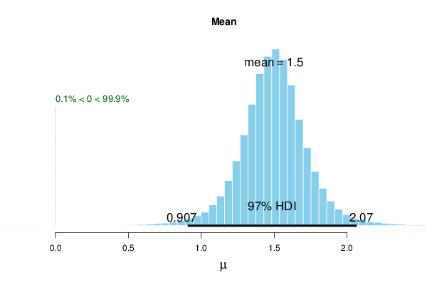
Figure 122.1: Bayesian Two Sample Test (paired, uninformative)

The above example shows the results for uninformative priors with paired samples. The mean difference (\(\simeq 1.497\)) has a 97% highest-density interval (HDI) that does not contain zero, and the posterior probability that the effect exceeds zero is very high (%>compVal = 99.9). For comparison, the Paired Two Sample t-Test yields a narrower frequentist confidence interval: [1.020,1.956].

If we assume unpaired samples and recompute the Bayesian Two Sample Test we should see an HDI which is wider than in the case with paired samples.

Table 122.2: Bayesian Two Sample Test (unpaired, uninformative)

	mean	median	mode	HDI%	HDIlo	HDIup	compVal	%>compVal
mu1	4.688	4.684	4.645	97	3.5921	5.83
mu2	3.214	3.220	3.254	97	2.3094	4.10
muDiff	1.474	1.470	1.474	97	0.0585	2.88	0	98.8
sigma1	1.022	0.890	0.719	97	0.3355	2.32
sigma2	0.832	0.728	0.609	97	0.2836	1.88
sigmaDiff	0.189	0.153	0.124	97	-1.4366	1.90	0	64.1
nu	33.636	25.168	8.815	97	1.0098	106.92
log10nu	1.363	1.401	1.506	97	0.4647	2.16
effSz	1.702	1.685	1.667	97	0.0228	3.45	0	98.8

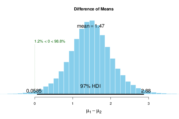
Figure 122.2: Bayesian Two Sample Test (unpaired, uninformative)

The results for the unpaired samples show strong posterior evidence of a positive mean difference because \(0 \notin [0.0585, 2.88]\) (97% HDI) and %>compVal = 98.8.

Again, it is possible to compare these results with the traditional Unpaired Two Sample t-Test which results in a 97% confidence interval of [0.489,2.488].

The difference between intervals for the unpaired samples case is rather substantial. For this reason we investigate what would happen if we had expert knowledge available (e.g. from previous studies). Let us suppose that the sample means correspond very well with the prior information that is available. We would specify the prior parameters \(\mu_{1,prior} = 4.688\) and \(\mu_{2,prior} = 3.214\).

In addition, assume that the standard deviations from both samples are believed to be (approximately) 0.7, i.e. smaller than those that were used in the uninformative case where \(\sigma_{1,prior} = 5 \times 1.022\) and \(\sigma_{2,prior} = 5 \times 0.832\).

The results from the Bayesian Two Sample Test with informative priors is shown below:

Table 122.3: Bayesian Two Sample Test (unpaired, informative)

	mean	median	mode	HDI%	HDIlo	HDIup	compVal	%>compVal
mu1	4.690	4.690	4.702	97	3.898	5.45
mu2	3.216	3.217	3.242	97	2.536	3.89
muDiff	1.474	1.475	1.492	97	0.467	2.48	0	99.9
sigma1	0.938	0.879	0.776	97	0.405	1.71
sigma2	0.776	0.721	0.636	97	0.323	1.46
sigmaDiff	0.162	0.153	0.175	97	-0.790	1.19	0	66.6
nu	34.314	25.655	10.097	97	1.002	108.38
log10nu	1.376	1.409	1.455	97	0.488	2.14
effSz	1.776	1.745	1.741	97	0.392	3.29	0	99.9

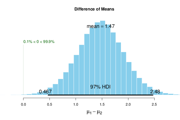
Table 122.4: Bayesian Two Sample Test (unpaired, informative)

The 97% HDI of the Bayesian method (with informative priors) is now very close to the interval of the traditional method. We conclude that the Bayesian Two Sample Test encompasses the traditional t-Test framework while making prior beliefs explicit and probabilistic.

To compute the Bayesian Two Sample Test on your local machine, the following script can be used in the R console:

library(BEST)
set.seed(123)
A <- rnorm(15)
B <- rnorm(15)
z <- cbind(A, B)
par1 = 1 #column number of first sample
par2 = 2 #column number of second sample
par3 = 0 #Null Hypothesis H0 
par4 = 0.95 #posterior credible mass (HDI)
par5 = 'unpaired' #Are observations paired? 
par6 = 'no' #Use informative priors? 
par7 = '' #prior value of mu1
par8 = '' #prior value of mu2
par9 = '' #prior value of sigma 1 of the population mean
par10 = '' #prior value of sigma 2 of the population mean
par11 = '' #prior value of the mode of sigma 1
par12 = '' #prior value of the mode of sigma 2
par13 = '' #prior value of SD of sigma 1 
par14 = '' #prior value of SD of sigma 2
par15 = '' #prior value of normality parameter
par16 = '' #prior value of SD of normality parameter
if(par6=='no') {
  if(par5=='unpaired') {
    (r <- BESTmcmc(z[,par1], z[,par2], parallel=F))
  }
  if(par5=='paired') {
    (r <- BESTmcmc(z[,par1]-z[,par2], parallel=F))
  }
} else {
  yy <- cbind(z[1,],z[2,])
  if(par5=='unpaired') {
    (r <- BESTmcmc(z[,par1], z[,par2], priors=list(muM = c(par7,par8), muSD = c(par9,par10), sigmaMode = c(par11,par12), sigmaSD = c(par13, par14), nuMean = par15, nuSD = par16), parallel=F))
  }
  if(par5=='paired') {
    (r <- BESTmcmc(z[,par1]-z[,par2], priors=list(muM = c(par7,par8), muSD = c(par9,par10), sigmaMode = c(par11,par12), sigmaSD = c(par13,par14), nuMean = par15, nuSD = par16), parallel=F))
  }
}
summary(r, credMass=par4, compValeff=par3)
plot(r, credMass=par4, compVal=par3)

Note: the BEST library requires the installation of JAGS which can be obtained from https://sourceforge.net/projects/mcmc-jags/.

122.3 Assumptions

Bayesian methods do not make deterministic assumptions about the model parameters because one explicitly takes into account the a priori distribution. If high quality prior information is available, Bayesian methods tend to outperform traditional methods. If the priors are inaccurate, the result from Bayesian test will be farther from the truth than in traditional Hypothesis Testing.

Generally speaking, Bayesian methods seem to be more robust (i.e. less sensitive to outliers) than the traditional approaches.

122.4 Alternatives

The alternative of this test are explained in Section 118.4.