The Exponential distribution answers a single practical question: how long until the next event? Whenever events occur at a constant average rate — equipment failures, customer arrivals, radioactive decays — the gap between them follows an Exponential distribution.
Formally, the random variate \(X\) defined for the range \(X \in [0, \infty)\), is said to have an Exponential Distribution (i.e. \(X \sim \text{Exp}(\lambda)\)) with rate parameter \(\lambda > 0\).
Parameterization note. Some texts use the mean parameter \(\beta = 1/\lambda\) (so that \(\text{E}(X) = \beta\) directly). Exponential functions in base R (dexp, pexp, qexp, rexp) use rate; to work with scale \(\beta = 1/\lambda\), pass rate = 1/beta. Throughout this chapter we use the rate parameterization \(\lambda\).
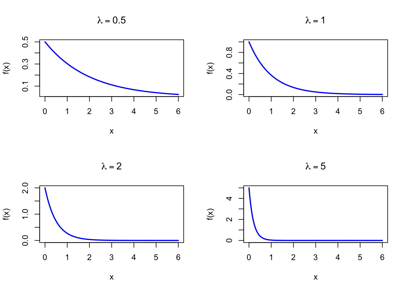
The figure below shows examples of the Exponential Probability Density Function for different values of \(\lambda\).
Code
par(mfrow =c(2, 2))x <-seq(0, 6, length =500)plot(x, dexp(x, rate =0.5), type ="l", lwd =2, col ="blue",xlab ="x", ylab ="f(x)", main =expression(lambda ==0.5))plot(x, dexp(x, rate =1), type ="l", lwd =2, col ="blue",xlab ="x", ylab ="f(x)", main =expression(lambda ==1))plot(x, dexp(x, rate =2), type ="l", lwd =2, col ="blue",xlab ="x", ylab ="f(x)", main =expression(lambda ==2))plot(x, dexp(x, rate =5), type ="l", lwd =2, col ="blue",xlab ="x", ylab ="f(x)", main =expression(lambda ==5))par(mfrow =c(1, 1))
Figure 27.1: Exponential Probability Density Function for various values of lambda
27.2 Purpose
The Exponential distribution is used to model waiting times and lifetimes when the rate of events is constant over time — equivalently, when the probability of an event in the next small interval does not depend on how much time has already elapsed (the memoryless property). Common applications include:
Time between successive events in a Poisson process (interarrival times)
Time to failure in reliability engineering (electronic components, machinery)
Duration of telephone calls and customer service interactions
Response and service times in queuing models
Radioactive decay times in nuclear physics
Relation to the discrete setting. The Exponential distribution is the continuous analog of the Geometric distribution — both share the memoryless property. Where the Geometric counts the number of discrete Bernoulli trials until the first success, the Exponential measures the continuous waiting time until the first event in a Poisson process. In both cases, past history provides no information about future waiting: the process always “starts fresh.” Both distributions have a coefficient of variation equal to 1.
27.3 Distribution Function
\[
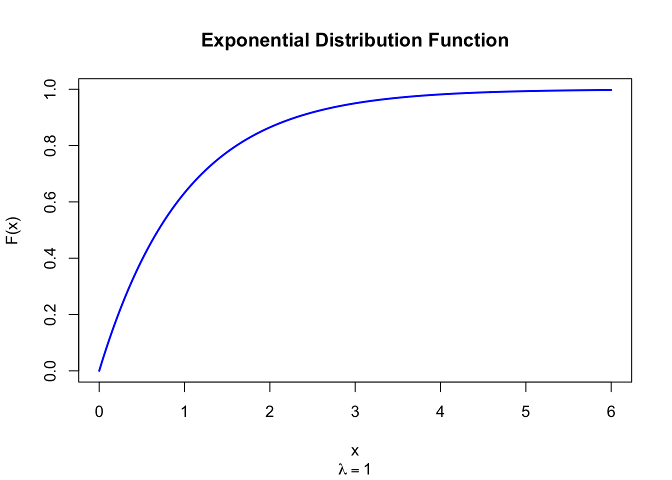
F(x) = 1 - e^{-\lambda x}, \quad x \geq 0
\]
The figure below shows the Exponential Distribution Function for \(\lambda = 1\).
Code
x <-seq(0, 6, length =500)plot(x, pexp(x, rate =1), type ="l", lwd =2, col ="blue",xlab ="x", ylab ="F(x)", main ="Exponential Distribution Function",sub =expression(lambda ==1))
Figure 27.2: Exponential Distribution Function (lambda = 1)
Note that \(1/\hat{\lambda} = \bar{x}\) is an unbiased estimator of \(1/\lambda = \text{E}(X)\). However, \(\hat{\lambda}\) itself is biased for \(\lambda\); the minimum-variance unbiased estimator of \(\lambda\) is \((n-1)/(n\bar{x})\).
27.19 R Module
27.19.1 RFC
The Exponential Distribution module is available in RFC under the menu “Distributions / Exponential Distribution”.
A data center monitors server uptime before hardware failure. Based on historical records, the mean time between failures (MTBF) is 200 hours, corresponding to a failure rate of \(\lambda = 1/200 = 0.005\) failures per hour. We model the time to failure as \(X \sim \text{Exp}(0.005)\).
lambda <-0.005# P(X <= 100): server fails within the first 100 hourscat("P(failure within 100 h):", pexp(100, rate = lambda), "\n")# P(X > 500): server survives beyond 500 hourscat("P(survives beyond 500 h):", 1-pexp(500, rate = lambda), "\n")# Median time to failurecat("Median time to failure (h):", qexp(0.5, rate = lambda), "\n")# 90th percentile: 90% of failures occur before this timecat("90th percentile (h):", qexp(0.9, rate = lambda), "\n")
P(failure within 100 h): 0.3934693
P(survives beyond 500 h): 0.082085
Median time to failure (h): 138.6294
90th percentile (h): 460.517
You can reproduce this exact scenario with the preconfigured Exponential app:
Exponential random variates can be generated from uniform random numbers via the inverse-CDF (probability integral transform). Since \(F(x) = 1 - e^{-\lambda x}\), setting \(U = F(X)\) and solving for \(X\) gives:
\[
X = -\frac{\ln(1 - U)}{\lambda} \sim \text{Exp}(\lambda) \quad \text{when } U \sim \text{U}(0,1)
\]
Because \(1 - U\) is also uniform on \((0,1)\), the equivalent form \(X = -\ln(U)/\lambda\) is commonly used.
set.seed(123)n <-1000lambda <-1# Inverse-transform methodu <-runif(n)x_inv <--log(u) / lambda# Built-in functionx_rexp <-rexp(n, rate = lambda)cat("Inverse-transform: mean =", round(mean(x_inv), 4)," var =", round(var(x_inv), 4), "\n")cat("rexp(): mean =", round(mean(x_rexp), 4)," var =", round(var(x_rexp), 4), "\n")cat("Theoretical: mean =", 1/lambda," var =", 1/lambda^2, "\n")
Inverse-transform: mean = 1.0064   var = 1.016
rexp():            mean = 1.0331   var = 1.0425
Theoretical:       mean = 1   var = 1
Code
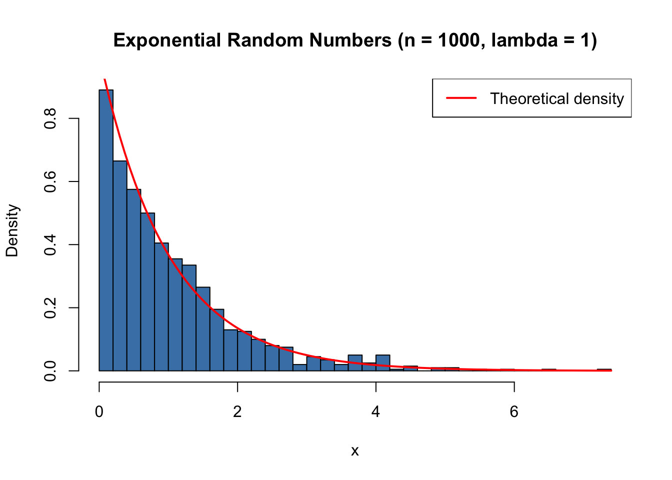
set.seed(123)x <-rexp(1000, rate =1)hist(x, breaks =30, col ="steelblue", freq =FALSE,xlab ="x", main ="Exponential Random Numbers (n = 1000, lambda = 1)")curve(dexp(x, rate =1), add =TRUE, col ="red", lwd =2)legend("topright", legend ="Theoretical density", col ="red", lwd =2)
Figure 27.3: Histogram of simulated Exponential random numbers (n = 1000, lambda = 1)
The Exponential distribution is the only continuous distribution with the memoryless property:
\[
\text{P}(X > s + t \mid X > s) = \text{P}(X > t) \quad \text{for all } s, t \geq 0
\]
Intuitively, if a server has already been running for \(s\) hours without failure, the distribution of remaining uptime is identical to the original distribution. Past survival provides no information about future failure.
27.23 Property 2: Minimum of Independent Exponentials
If \(X_1 \sim \text{Exp}(\lambda_1)\) and \(X_2 \sim \text{Exp}(\lambda_2)\) are independent, then their minimum is also exponentially distributed:
More generally, the minimum of \(n\) independent exponentials with rates \(\lambda_1, \ldots, \lambda_n\) follows \(\text{Exp}(\lambda_1 + \cdots + \lambda_n)\).
27.24 Property 3: Coefficient of Variation Equals 1
The coefficient of variation (CV = standard deviation / mean) is always exactly 1:
This holds for every value of \(\lambda\). An observed CV substantially different from 1 suggests the Exponential model may not be appropriate for the data.
27.25 Related Distributions 1: Special Case of Gamma
The Exponential distribution is a special case of the Gamma distribution with shape parameter equal to 1 (see Chapter 29):
27.26 Related Distributions 2: Interarrival Times in a Poisson Process
In a Poisson process with rate \(\lambda\), the times between consecutive events (interarrival times) are independent and identically distributed as \(\text{Exp}(\lambda)\) (see Chapter 18). Conversely, if interarrival times are i.i.d. \(\text{Exp}(\lambda)\), the count of events in any fixed interval follows \(\text{Pois}(\lambda \cdot \text{interval length})\).