• Descriptive
    • Moments
    • Concentration
    • Central Tendency
    • Variability
    • Stem-and-Leaf Plot
    • Histogram & Frequency Table
    • Data Quality Forensics
    • Conditional EDA
    • Quantiles
    • Kernel Density Estimation
    • Normal QQ Plot
    • Bootstrap Plot

    • Multivariate Descriptive Statistics
  • Distributions
    • Binomial Probabilities
    • Geometric Probabilities
    • Negative Binomial Probabilities
    • Hypergeometric Probabilities
    • Multinomial Probabilities
    • Poisson Probabilities

    • Exponential
    • Gamma
    • Erlang
    • Weibull
    • Rayleigh
    • Lognormal
    • Pareto
    • Inverse Gamma

    • Beta
    • Power
    • Beta Prime (Inv. Beta)
    • Triangular

    • Normal (area)
    • Logistic
    • Laplace
    • Cauchy (standard)
    • Cauchy (location-scale)
    • Gumbel

    • Normal RNG
    • ML Fitting
    • Tukey Lambda PPCC
    • Box-Cox Normality Plot
    • Sample Correlation r

    • Empirical Tests
  • Hypotheses
    • Theoretical Aspects of Hypothesis Testing
    • Bayesian Inference
    • Minimum Sample Size

    • Empirical Tests
    • Multivariate (pair-wise) Testing
  • Models
    • Manual Model Building
  • Time Series
    • Time Series Plot
    • Decomposition
    • Exponential Smoothing

    • Blocked Bootstrap Plot
    • Mean Plot
    • (P)ACF
    • VRM
    • Standard Deviation-Mean Plot
    • Spectral Analysis
    • ARIMA

    • Cross Correlation Function
    • Granger Causality
  1. Probability Distributions
  2. 38  Gumbel Distribution
  • Preface
  • Getting Started
    • 1  Introduction
    • 2  Why Do We Need Innovative Technology?
    • 3  Basic Definitions
    • 4  The Big Picture: Why We Analyze Data
  • Introduction to Probability
    • 5  Definitions of Probability
    • 6  Jeffreys’ axiom system
    • 7  Bayes’ Theorem
    • 8  Sensitivity and Specificity
    • 9  Naive Bayes Classifier
    • 10  Law of Large Numbers

    • 11  Problems
  • Probability Distributions
    • 12  Bernoulli Distribution
    • 13  Binomial Distribution
    • 14  Geometric Distribution
    • 15  Negative Binomial Distribution
    • 16  Hypergeometric Distribution
    • 17  Multinomial Distribution
    • 18  Poisson Distribution

    • 19  Uniform Distribution (Rectangular Distribution)
    • 20  Normal Distribution (Gaussian Distribution)
    • 21  Gaussian Naive Bayes Classifier
    • 22  Chi Distribution
    • 23  Chi-squared Distribution (1 parameter)
    • 24  Chi-squared Distribution (2 parameters)
    • 25  Student t-Distribution
    • 26  Fisher F-Distribution
    • 27  Exponential Distribution
    • 28  Lognormal Distribution
    • 29  Gamma Distribution
    • 30  Beta Distribution
    • 31  Weibull Distribution
    • 32  Pareto Distribution
    • 33  Inverse Gamma Distribution
    • 34  Rayleigh Distribution
    • 35  Erlang Distribution
    • 36  Logistic Distribution
    • 37  Laplace Distribution
    • 38  Gumbel Distribution
    • 39  Cauchy Distribution
    • 40  Triangular Distribution
    • 41  Power Distribution
    • 42  Beta Prime Distribution
    • 43  Sample Correlation Distribution

    • 44  Problems
  • Descriptive Statistics & Exploratory Data Analysis
    • 45  Types of Data
    • 46  Datasheets

    • 47  Frequency Plot (Bar Plot)
    • 48  Frequency Table
    • 49  Contingency Table
    • 50  Binomial Classification Metrics
    • 51  Confusion Matrix
    • 52  ROC Analysis

    • 53  Stem-and-Leaf Plot
    • 54  Histogram
    • 55  Data Quality Forensics
    • 56  Quantiles
    • 57  Central Tendency
    • 58  Variability
    • 59  Skewness & Kurtosis
    • 60  Concentration
    • 61  Notched Boxplot
    • 62  Scatterplot
    • 63  Pearson Correlation
    • 64  Rank Correlation
    • 65  Partial Pearson Correlation
    • 66  Simple Linear Regression
    • 67  Moments
    • 68  Quantile-Quantile Plot (QQ Plot)
    • 69  Normal Probability Plot
    • 70  Probability Plot Correlation Coefficient Plot (PPCC Plot)
    • 71  Box-Cox Normality Plot
    • 72  Kernel Density Estimation
    • 73  Bivariate Kernel Density Plot
    • 74  Conditional EDA: Panel Diagnostics
    • 75  Bootstrap Plot (Central Tendency)
    • 76  Survey Scores Rank Order Comparison
    • 77  Cronbach Alpha

    • 78  Equi-distant Time Series
    • 79  Time Series Plot (Run Sequence Plot)
    • 80  Mean Plot
    • 81  Blocked Bootstrap Plot (Central Tendency)
    • 82  Standard Deviation-Mean Plot
    • 83  Variance Reduction Matrix
    • 84  (Partial) Autocorrelation Function
    • 85  Periodogram & Cumulative Periodogram

    • 86  Problems
  • Hypothesis Testing
    • 87  Normal Distributions revisited
    • 88  The Population
    • 89  The Sample
    • 90  The One-Sided Hypothesis Test
    • 91  The Two-Sided Hypothesis Test
    • 92  When to use a one-sided or two-sided test?
    • 93  What if \(\sigma\) is unknown?
    • 94  The Central Limit Theorem (revisited)
    • 95  Statistical Test of the Population Mean with known Variance
    • 96  Statistical Test of the Population Mean with unknown Variance
    • 97  Statistical Test of the Variance
    • 98  Statistical Test of the Population Proportion
    • 99  Statistical Test of the Standard Deviation \(\sigma\)
    • 100  Statistical Test of the difference between Means -- Independent/Unpaired Samples
    • 101  Statistical Test of the difference between Means -- Dependent/Paired Samples
    • 102  Statistical Test of the difference between Variances -- Independent/Unpaired Samples

    • 103  Hypothesis Testing for Research Purposes
    • 104  Decision Thresholds, Alpha, and Confidence Levels
    • 105  Bayesian Inference for Decision-Making
    • 106  One Sample t-Test
    • 107  Skewness & Kurtosis Tests
    • 108  Paired Two Sample t-Test
    • 109  Wilcoxon Signed-Rank Test
    • 110  Unpaired Two Sample t-Test
    • 111  Unpaired Two Sample Welch Test
    • 112  Two One-Sided Tests (TOST) for Equivalence
    • 113  Mann-Whitney U test (Wilcoxon Rank-Sum Test)
    • 114  Bayesian Two Sample Test
    • 115  Median Test based on Notched Boxplots
    • 116  Chi-Squared Tests for Count Data
    • 117  Kolmogorov-Smirnov Test
    • 118  One Way Analysis of Variance (1-way ANOVA)
    • 119  Kruskal-Wallis Test
    • 120  Two Way Analysis of Variance (2-way ANOVA)
    • 121  Repeated Measures ANOVA
    • 122  Friedman Test
    • 123  Testing Correlations
    • 124  A Note on Causality

    • 125  Problems
  • Regression Models
    • 126  Simple Linear Regression Model (SLRM)
    • 127  Multiple Linear Regression Model (MLRM)
    • 128  Logistic Regression
    • 129  Generalized Linear Models
    • 130  Multinomial and Ordinal Logistic Regression
    • 131  Cox Proportional Hazards Regression
    • 132  Conditional Inference Trees
    • 133  Leaf Diagnostics for Conditional Inference Trees
    • 134  Hypothesis Testing with Linear Regression Models (from a Practical Point of View)

    • 135  Problems
  • Introduction to Time Series Analysis
    • 136  Case: the Market of Health and Personal Care Products
    • 137  Decomposition of Time Series
    • 138  Ad hoc Forecasting of Time Series
  • Box-Jenkins Analysis
    • 139  Introduction to Box-Jenkins Analysis
    • 140  Theoretical Concepts
    • 141  Stationarity
    • 142  Identifying ARMA parameters
    • 143  Estimating ARMA Parameters and Residual Diagnostics
    • 144  Forecasting with ARIMA models
    • 145  Intervention Analysis
    • 146  Cross-Correlation Function
    • 147  Transfer Function Noise Models
    • 148  General-to-Specific Modeling
  • References
  • Appendices
    • Appendices
    • A  Method Selection Guide
    • B  Presentations and Teaching Materials
    • C  R Language Concepts for Statistical Computing
    • D  Matrix Algebra
    • E  Standard Normal Table (Gaussian Table)
    • F  Critical values of Student’s \(t\) distribution with \(\nu\) degrees of freedom
    • G  Upper-tail critical values of the \(\chi^2\)-distribution with \(\nu\) degrees of freedom
    • H  Lower-tail critical values of the \(\chi^2\)-distribution with \(\nu\) degrees of freedom

Table of contents

  • 38.1 Probability Density Function
  • 38.2 Purpose
  • 38.3 Distribution Function
  • 38.4 Moment Generating Function
  • 38.5 1st Uncentered Moment
  • 38.6 2nd Uncentered Moment
  • 38.7 3rd Uncentered Moment
  • 38.8 4th Uncentered Moment
  • 38.9 2nd Centered Moment
  • 38.10 3rd Centered Moment
  • 38.11 4th Centered Moment
  • 38.12 Expected Value
  • 38.13 Variance
  • 38.14 Median
  • 38.15 Mode
  • 38.16 Coefficient of Skewness
  • 38.17 Coefficient of Kurtosis
  • 38.18 Parameter Estimation
  • 38.19 R Module
    • 38.19.1 RFC
    • 38.19.2 Direct app link
    • 38.19.3 R Code
  • 38.20 Example
  • 38.21 Random Number Generator
  • 38.22 Property 1: Fisher-Tippett-Gnedenko Theorem
  • 38.23 Property 2: Universal Shape Constants
  • 38.24 Property 3: Relationship to Weibull via Minimum
  • 38.25 Related Distributions 1: Weibull Distribution
  • 38.26 Related Distributions 2: Exponential Distribution
DRAFT This draft is under development — DO NOT CITE OR SHARE.
  1. Probability Distributions
  2. 38  Gumbel Distribution

38  Gumbel Distribution

The Gumbel distribution is the limiting distribution of the maximum of many independent random variables from light-tailed distributions. It is the cornerstone of extreme-value statistics, used wherever one needs to model the probability of record-breaking events: annual flood peaks, maximum daily temperatures, or largest structural loads.

Formally, the random variate \(X\) defined for all of \(\mathbb{R}\), is said to have a Gumbel Distribution (i.e. \(X \sim \text{Gumbel}(\mu, \beta)\)) with location parameter \(\mu \in \mathbb{R}\) and scale parameter \(\beta > 0\). The Euler-Mascheroni constant is \(\gamma \approx 0.5772156649\).

38.1 Probability Density Function

\[ f(x) = \frac{1}{\beta}\exp\!\bigl(-z - e^{-z}\bigr), \quad z = \frac{x - \mu}{\beta} \]

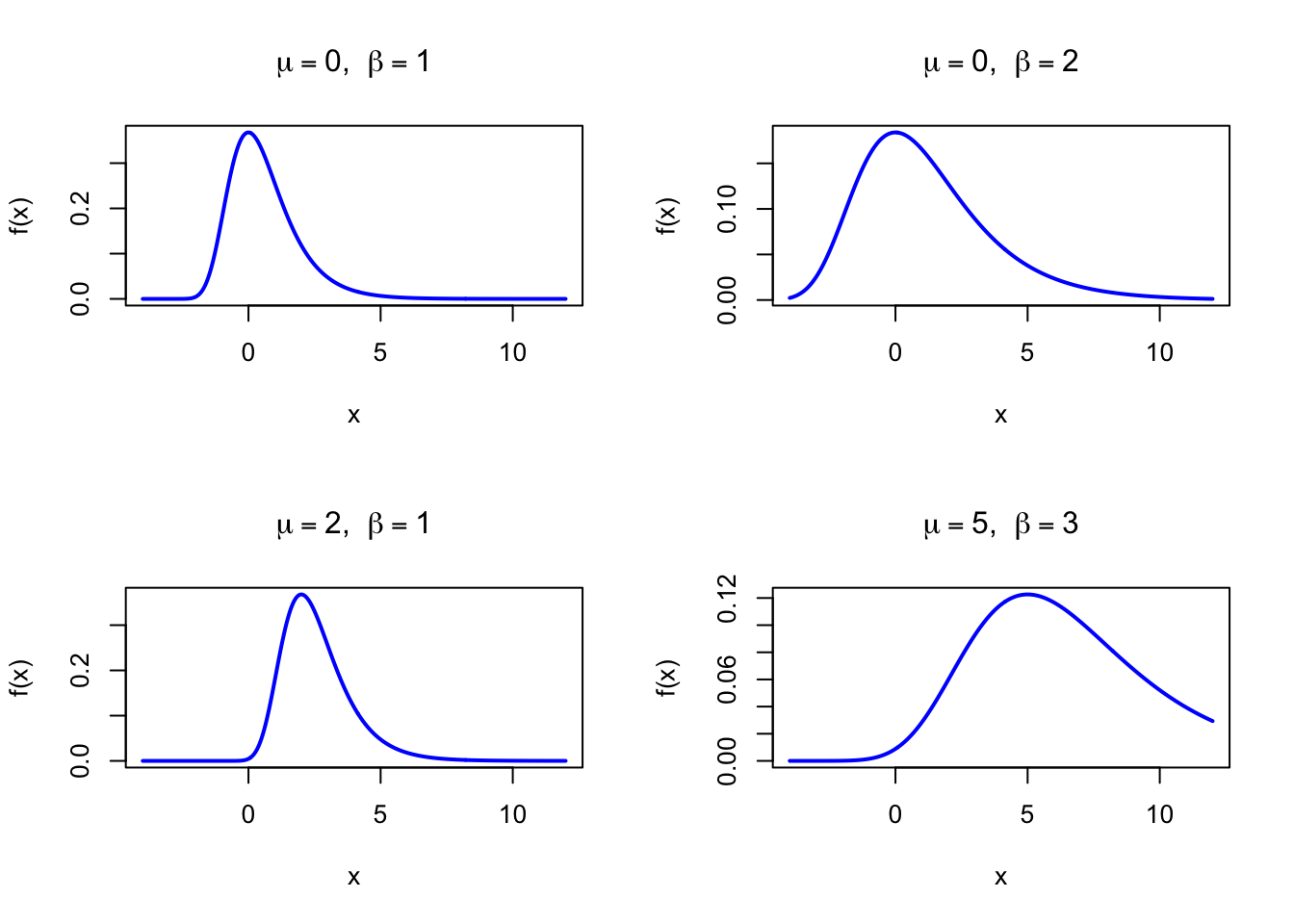
The figure below shows examples of the Gumbel Probability Density Function for different parameter combinations.

Code
dgumbel <- function(x, mu, beta) {
  z <- (x - mu) / beta
  exp(-z - exp(-z)) / beta
}

par(mfrow = c(2, 2))
x <- seq(-4, 12, length = 500)

plot(x, dgumbel(x, 0, 1), type = "l", lwd = 2, col = "blue",
     xlab = "x", ylab = "f(x)", main = expression(paste(mu == 0, ",  ", beta == 1)))

plot(x, dgumbel(x, 0, 2), type = "l", lwd = 2, col = "blue",
     xlab = "x", ylab = "f(x)", main = expression(paste(mu == 0, ",  ", beta == 2)))

plot(x, dgumbel(x, 2, 1), type = "l", lwd = 2, col = "blue",
     xlab = "x", ylab = "f(x)", main = expression(paste(mu == 2, ",  ", beta == 1)))

plot(x, dgumbel(x, 5, 3), type = "l", lwd = 2, col = "blue",
     xlab = "x", ylab = "f(x)", main = expression(paste(mu == 5, ",  ", beta == 3)))

par(mfrow = c(1, 1))
Figure 38.1: Gumbel Probability Density Function for various parameter combinations

38.2 Purpose

The Gumbel distribution belongs to the generalized extreme value (GEV) family and specifically describes the limiting distribution of block maxima from distributions with exponentially bounded tails (Normal, Exponential, Gamma). Its right-skewed shape with a mode below the mean is characteristic of maximum-type data. Common applications include:

  • Hydrology: annual maximum flood discharge, maximum daily rainfall
  • Structural engineering: maximum wind load, maximum snow depth for design standards
  • Climatology: maximum daily temperature records, extreme precipitation events
  • Financial risk: maximum portfolio loss within a given time horizon
  • Reliability engineering: maximum stress or load applied to a component

Relation to the discrete setting. The Gumbel distribution is the continuous limit of the maximum of \(n\) i.i.d. Geometric or Poisson variates after normalization — the Fisher-Tippett-Gnedenko theorem applies in the discrete domain too. For the maximum of Geometric\((p)\) variates as \(n\to\infty\), the normalized maximum approaches a Gumbel distribution.

38.3 Distribution Function

\[ F(x) = \exp\!\bigl(-e^{-(x-\mu)/\beta}\bigr) \]

The figure below shows the Gumbel Distribution Function for \(\mu = 0\) and \(\beta = 1\).

Code
pgumbel <- function(x, mu, beta) {
  exp(-exp(-(x - mu) / beta))
}

x <- seq(-4, 10, length = 500)
plot(x, pgumbel(x, 0, 1), type = "l", lwd = 2, col = "blue",
     xlab = "x", ylab = "F(x)", main = "Gumbel Distribution Function",
     sub = expression(paste(mu == 0, ",  ", beta == 1)))
Figure 38.2: Gumbel Distribution Function (location = 0, scale = 1)

38.4 Moment Generating Function

\[ M_X(t) = \Gamma(1 - \beta t)\,e^{\mu t}, \quad t < \frac{1}{\beta} \]

where \(\gamma \approx 0.5772156649\) is the Euler-Mascheroni constant and \(\Gamma(\cdot)\) is the gamma function.

38.5 1st Uncentered Moment

\[ \mu_1' = \mu + \gamma\beta \]

where \(\gamma \approx 0.5772156649\) is the Euler-Mascheroni constant.

38.6 2nd Uncentered Moment

\[ \mu_2' = (\mu + \gamma\beta)^2 + \frac{\pi^2\beta^2}{6} \]

38.7 3rd Uncentered Moment

Obtained via the third derivative of the MGF; involves the polygamma function \(\psi''(1) = -2\zeta(3)\) where \(\zeta(3) \approx 1.20206\).

38.8 4th Uncentered Moment

Obtained via the fourth derivative of the MGF.

38.9 2nd Centered Moment

\[ \mu_2 = \frac{\pi^2\beta^2}{6} \]

38.10 3rd Centered Moment

\[ \mu_3 = 2\zeta(3)\beta^3, \quad \zeta(3) \approx 1.20206 \]

38.11 4th Centered Moment

\[ \mu_4 = \frac{27}{5}\,\mu_2^2 = \frac{27}{5}\cdot\frac{\pi^4\beta^4}{36} \]

38.12 Expected Value

\[ \text{E}(X) = \mu + \gamma\beta, \quad \gamma \approx 0.5772156649 \]

38.13 Variance

\[ \text{V}(X) = \frac{\pi^2\beta^2}{6} \]

38.14 Median

\[ \text{Med}(X) = \mu - \beta\ln(\ln 2) \]

38.15 Mode

\[ \text{Mo}(X) = \mu \]

38.16 Coefficient of Skewness

\[ g_1 = \frac{12\sqrt{6}\,\zeta(3)}{\pi^3} \approx 1.1395 \]

This is a fixed universal constant, independent of \(\mu\) and \(\beta\).

38.17 Coefficient of Kurtosis

\[ g_2 = \frac{27}{5} = 5.4 \]

This is also a fixed universal constant. The excess kurtosis is \(g_2 - 3 = 2.4\).

38.18 Parameter Estimation

Method-of-moments estimates from mean and variance:

\[ \tilde\beta = \frac{s\sqrt{6}}{\pi}, \qquad \tilde\mu = \bar x - \gamma\tilde\beta \]

where \(s\) is the sample standard deviation and \(\gamma \approx 0.5772\).

set.seed(42)
mu_true <- 10; beta_true <- 5
u <- runif(100)
x_obs <- mu_true - beta_true * log(-log(u))

# Method of moments
gamma_em <- 0.5772156649
beta_hat <- sd(x_obs) * sqrt(6) / pi
mu_hat   <- mean(x_obs) - gamma_em * beta_hat
cat("MoM mu:  ", round(mu_hat, 4), "\n")
cat("MoM beta:", round(beta_hat, 4), "\n")
cat("True mu:", mu_true, "  True beta:", beta_true, "\n")
MoM mu:   10.2689 
MoM beta: 5.3249 
True mu: 10   True beta: 5 

38.19 R Module

38.19.1 RFC

The Gumbel Distribution module is available in RFC under the menu “Distributions / Gumbel Distribution”.

38.19.2 Direct app link

  • https://shiny.wessa.net/gumbel/

38.19.3 R Code

The following code demonstrates Gumbel probability calculations:

mu <- 10; beta <- 5
gamma_em <- 0.5772156649

dgumbel <- function(x, mu, beta) {
  z <- (x - mu) / beta
  exp(-z - exp(-z)) / beta
}
pgumbel <- function(x, mu, beta) exp(-exp(-(x - mu) / beta))

# P(X <= 18)
pgumbel(18, mu, beta)

# P(X > 18)
1 - pgumbel(18, mu, beta)

# Mean and mode
cat("Mean:", mu + gamma_em * beta, "\n")
cat("Mode:", mu, "\n")
cat("Median:", mu - beta * log(log(2)), "\n")
[1] 0.8171795
[1] 0.1828205
Mean: 12.88608 
Mode: 10 
Median: 11.83256 

38.20 Example

Annual maximum wind gust speeds (m/s) at a weather station are modeled as \(X \sim \text{Gumbel}(\mu = 10, \beta = 5)\). We compute the probability that the annual maximum gust exceeds 18 m/s.

mu <- 10; beta <- 5
gamma_em <- 0.5772156649
pgumbel <- function(x, mu, beta) exp(-exp(-(x - mu) / beta))

# P(max gust > 18 m/s)
cat("P(max gust > 18 m/s):", 1 - pgumbel(18, mu, beta), "\n")

# Mean annual maximum
cat("Mean max gust (m/s):", mu + gamma_em * beta, "\n")

# 100-year return level: 99th percentile
x_100yr <- mu - beta * log(-log(0.99))
cat("100-year return level (m/s):", round(x_100yr, 2), "\n")
P(max gust > 18 m/s): 0.1828205 
Mean max gust (m/s): 12.88608 
100-year return level (m/s): 33 
Interactive Shiny app (click to load).
Open in new tab

38.21 Random Number Generator

Gumbel random variates are generated via the inverse-CDF method. Since \(F(x) = \exp(-e^{-(x-\mu)/\beta})\), solving for \(X\) gives:

\[ X = \mu - \beta\ln(-\ln U) \sim \text{Gumbel}(\mu, \beta) \quad \text{when } U \sim \text{U}(0,1) \]

set.seed(123)
n <- 1000; mu <- 0; beta <- 1
gamma_em <- 0.5772156649

# Inverse-transform method
u <- runif(n)
x_inv <- mu - beta * log(-log(u))

cat("Simulated mean:", round(mean(x_inv), 4), "\n")
cat("Theoretical mean:", mu + gamma_em * beta, "\n")
cat("Simulated var:", round(var(x_inv), 4), "\n")
cat("Theoretical var:", round(pi^2 * beta^2 / 6, 4), "\n")
Simulated mean: 0.561 
Theoretical mean: 0.5772157 
Simulated var: 1.5925 
Theoretical var: 1.6449 
Interactive Shiny app (click to load).
Open in new tab

38.22 Property 1: Fisher-Tippett-Gnedenko Theorem

The Gumbel distribution is one of only three possible limiting distributions for normalized block maxima (Fisher-Tippett-Gnedenko theorem). It arises from distributions with exponentially bounded tails (Normal, Gamma, Exponential, Lognormal). This is the continuous-data counterpart of the classical central limit theorem for extreme values.

38.23 Property 2: Universal Shape Constants

Both the skewness \(g_1 \approx 1.1395\) and kurtosis \(g_2 = 5.4\) are universal constants — they do not depend on \(\mu\) or \(\beta\). Any data with these shape properties is consistent with the Gumbel model.

38.24 Property 3: Relationship to Weibull via Minimum

If \(X \sim \text{Gumbel}(\mu, \beta)\) then \(-X\) follows the minimum (reversed) Gumbel distribution. Furthermore, if \(Y = e^{-X/\beta}\) then \(Y\) follows a Weibull distribution, linking the two extreme-value families.

38.25 Related Distributions 1: Weibull Distribution

The Weibull distribution is related to the Gumbel via a log-transformation: if \(X \sim \text{Weibull}(k, \lambda)\) then \(\ln\!\left((X/\lambda)^k\right)\) follows the minimum Gumbel, while \(-\ln\!\left((X/\lambda)^k\right)\) follows the maximum Gumbel (see Chapter 31).

38.26 Related Distributions 2: Exponential Distribution

The Exponential distribution belongs to the Gumbel domain of attraction: the normalized maximum of \(n\) i.i.d. Exp\((\lambda)\) variates converges to Gumbel as \(n \to \infty\) (see Chapter 27).

37  Laplace Distribution
39  Cauchy Distribution

© 2026 Patrick Wessa. Provided as-is, without warranty.

Feedback: e-mail | Anonymous contributions: click to copy (Sats) | click to copy (XMR)

Cookie Preferences