33  Inverse Gamma Distribution

The Inverse Gamma distribution is the distribution of the reciprocal of a Gamma random variable. In Bayesian statistics it is the standard conjugate prior for the variance \(\sigma^2\) of a Normal distribution, and it arises whenever one models precision or scale uncertainty.

Formally, the random variate \(X\) defined for the range \(X > 0\), is said to have an Inverse Gamma Distribution (i.e. \(X \sim \text{InvGamma}(\alpha, \beta)\)) with shape parameter \(\alpha > 0\) and scale parameter \(\beta > 0\). If \(Y \sim \text{Gamma}(\alpha, \beta)\) then \(X = 1/Y \sim \text{InvGamma}(\alpha, \beta)\).

33.1 Probability Density Function

\[ f(x) = \frac{\beta^\alpha}{\Gamma(\alpha)}\,x^{-\alpha-1}\exp(-\beta/x), \quad x > 0 \]

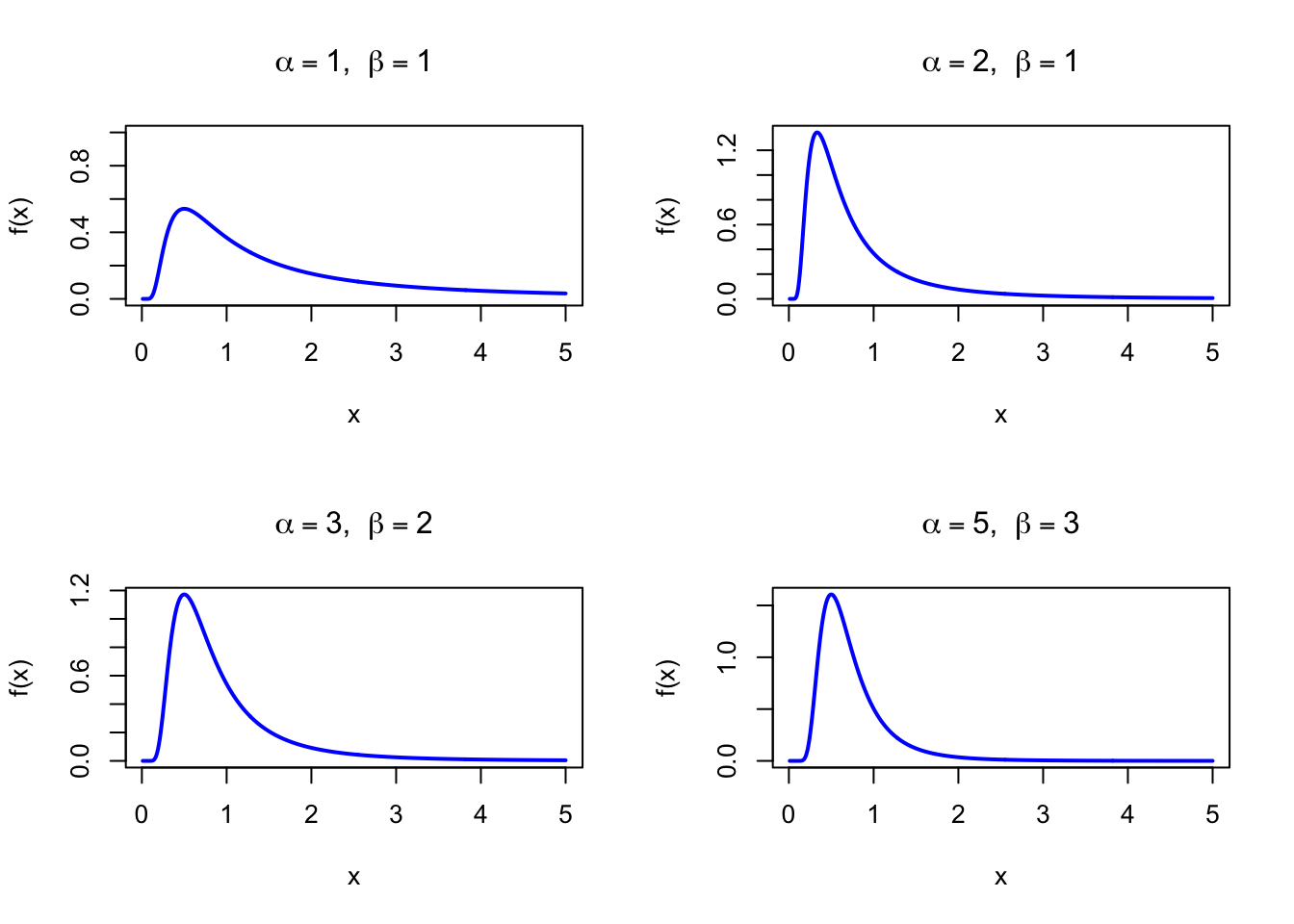
The figure below shows examples of the Inverse Gamma Probability Density Function for different parameter combinations.

dinvgamma <- function(x, alpha, beta) {
  ifelse(x > 0, beta^alpha / gamma(alpha) * x^(-alpha - 1) * exp(-beta / x), 0)
}

par(mfrow = c(2, 2))
x <- seq(0.01, 5, length = 500)

plot(x, dinvgamma(x, 1, 1), type = "l", lwd = 2, col = "blue",
     xlab = "x", ylab = "f(x)", main = expression(paste(alpha == 1, ",  ", beta == 1)),
     ylim = c(0, 1))

plot(x, dinvgamma(x, 2, 1), type = "l", lwd = 2, col = "blue",
     xlab = "x", ylab = "f(x)", main = expression(paste(alpha == 2, ",  ", beta == 1)))

plot(x, dinvgamma(x, 3, 2), type = "l", lwd = 2, col = "blue",
     xlab = "x", ylab = "f(x)", main = expression(paste(alpha == 3, ",  ", beta == 2)))

plot(x, dinvgamma(x, 5, 3), type = "l", lwd = 2, col = "blue",
     xlab = "x", ylab = "f(x)", main = expression(paste(alpha == 5, ",  ", beta == 3)))

par(mfrow = c(1, 1))

Figure 33.1: Inverse Gamma Probability Density Function for various parameter combinations

33.2 Purpose

The Inverse Gamma distribution arises naturally as the reciprocal of a Gamma random variable and plays a central role in Bayesian hierarchical modeling. Its most important application is as a conjugate prior for the variance parameter of a Normal likelihood. Common applications include:

• Bayesian prior for the variance \(\sigma^2\) in Normal-Normal models (conjugate prior)
• Posterior distribution of variance after observing Gaussian data
• Modeling scale or spread parameters that must be positive
• Scale-inverse-chi-squared distribution (reparameterized Inverse Gamma) in objective Bayes
• Mixing distribution in hierarchical models (e.g., Student’s t as Normal-Inverse-Gamma mixture)

Relation to the discrete setting. The Inverse Gamma has no direct discrete analog. Conceptually, it mirrors the Negative Binomial as a mixing distribution: just as a Poisson-Gamma mixture yields the Negative Binomial for counts, an analogous continuous hierarchy uses the Inverse Gamma to model scale uncertainty.

33.3 Distribution Function

\[ F(x) = \frac{\Gamma(\alpha,\,\beta/x)}{\Gamma(\alpha)}, \quad x > 0 \]

where \(\Gamma(\alpha, z) = \int_z^\infty t^{\alpha-1} e^{-t}\, dt\) is the upper incomplete gamma function. In R: pgamma(1/x, shape = alpha, rate = beta, lower.tail = FALSE) (note: Gamma rate = beta matches the InvGamma scale parameter \(\beta\)).

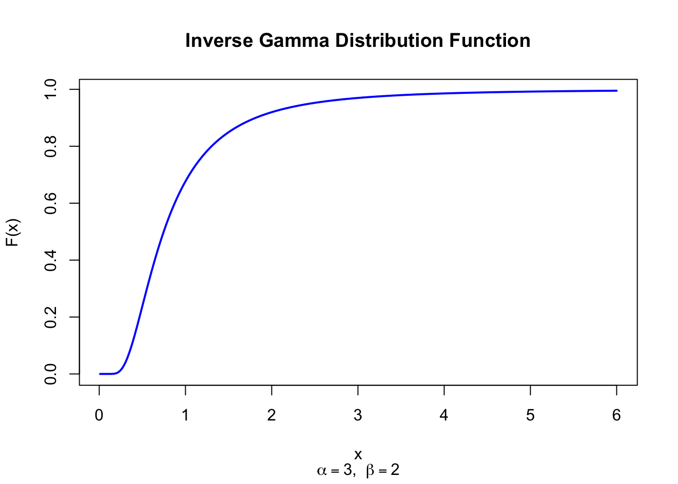
The figure below shows the Inverse Gamma Distribution Function for \(\alpha = 3\) and \(\beta = 2\).

pinvgamma <- function(x, alpha, beta) {
  pgamma(1/x, shape = alpha, rate = beta, lower.tail = FALSE)
}

x <- seq(0.01, 6, length = 500)
plot(x, pinvgamma(x, 3, 2), type = "l", lwd = 2, col = "blue",
     xlab = "x", ylab = "F(x)", main = "Inverse Gamma Distribution Function",
     sub = expression(paste(alpha == 3, ",  ", beta == 2)))

Figure 33.2: Inverse Gamma Distribution Function (alpha = 3, beta = 2)

33.4 Moment Generating Function

The moment generating function of the Inverse Gamma distribution does not exist for \(t > 0\).

33.5 1st Uncentered Moment

\[ \mu_1' = \frac{\beta}{\alpha - 1}, \quad \alpha > 1 \]

33.6 2nd Uncentered Moment

\[ \mu_2' = \frac{\beta^2}{(\alpha-1)(\alpha-2)}, \quad \alpha > 2 \]

33.7 3rd Uncentered Moment

\[ \mu_3' = \frac{\beta^3}{(\alpha-1)(\alpha-2)(\alpha-3)}, \quad \alpha > 3 \]

33.8 4th Uncentered Moment

\[ \mu_4' = \frac{\beta^4}{(\alpha-1)(\alpha-2)(\alpha-3)(\alpha-4)}, \quad \alpha > 4 \]

In general: \(\mu_n' = \dfrac{\beta^n\,\Gamma(\alpha-n)}{\Gamma(\alpha)}\) for \(n < \alpha\).

33.9 2nd Centered Moment

\[ \mu_2 = \frac{\beta^2}{(\alpha-1)^2(\alpha-2)}, \quad \alpha > 2 \]

33.10 3rd Centered Moment

Obtained by expanding raw moments; requires \(\alpha > 3\).

33.11 4th Centered Moment

Obtained by expanding raw moments; requires \(\alpha > 4\).

33.12 Expected Value

\[ \text{E}(X) = \frac{\beta}{\alpha - 1}, \quad \alpha > 1 \]

The mean is undefined for \(\alpha \leq 1\).

33.13 Variance

\[ \text{V}(X) = \frac{\beta^2}{(\alpha-1)^2(\alpha-2)}, \quad \alpha > 2 \]

33.14 Median

The median has no closed form and must be computed numerically:

# Median of InvGamma(alpha, beta): numerical
alpha <- 3; beta <- 2
pinvgamma <- function(x, alpha, beta) pgamma(1/x, shape = alpha, rate = beta, lower.tail = FALSE)
uniroot(function(x) pinvgamma(x, alpha, beta) - 0.5, c(0.001, 1000))$root

[1] 0.7479267

33.15 Mode

\[ \text{Mo}(X) = \frac{\beta}{\alpha + 1} \]

33.16 Coefficient of Skewness

\[ g_1 = \frac{4\sqrt{\alpha-2}}{\alpha-3}, \quad \alpha > 3 \]

The Inverse Gamma distribution is always positively skewed.

33.17 Coefficient of Kurtosis

\[ g_2 = 3 + \frac{30\alpha - 66}{(\alpha-3)(\alpha-4)}, \quad \alpha > 4 \]

33.18 Parameter Estimation

MLE is obtained numerically. Method-of-moments starting values:

\[ \tilde\alpha = \frac{\bar x^2}{s^2} + 2, \qquad \tilde\beta = \bar x\,(\tilde\alpha - 1) \]

# Simulate InvGamma(3, 2) data and estimate parameters
set.seed(42)
alpha_true <- 3; beta_true <- 2
x_sim <- 1 / rgamma(100, shape = alpha_true, rate = beta_true)

# Method-of-moments starting values
xbar <- mean(x_sim); s2 <- var(x_sim)
alpha_mom <- xbar^2 / s2 + 2
beta_mom  <- xbar * (alpha_mom - 1)
cat("MoM alpha:", round(alpha_mom, 4), "  MoM beta:", round(beta_mom, 4), "\n")
cat("True alpha:", alpha_true, "  True beta:", beta_true, "\n")

MoM alpha: 3.3236   MoM beta: 2.3767 
True alpha: 3   True beta: 2 

33.19 R Module

33.19.1 RFC

The Inverse Gamma Distribution module is available in RFC under the menu “Distributions / Inverse Gamma Distribution”.

33.19.2 Direct app link

• https://shiny.wessa.net/invgamma/

33.19.3 R Code

The following code demonstrates Inverse Gamma probability calculations:

alpha <- 3; beta <- 2

# Custom density function
dinvgamma <- function(x, alpha, beta) {
  ifelse(x > 0, beta^alpha / gamma(alpha) * x^(-alpha - 1) * exp(-beta / x), 0)
}

# Custom CDF using pgamma
pinvgamma <- function(x, alpha, beta) {
  pgamma(1/x, shape = alpha, rate = beta, lower.tail = FALSE)
}

# Density at x = 1
dinvgamma(1, alpha, beta)

# P(X <= 1): distribution function
pinvgamma(1, alpha, beta)

# Mode and mean
cat("Mode:", beta / (alpha + 1), "\n")
cat("Mean:", beta / (alpha - 1), "\n")

[1] 0.5413411
[1] 0.6766764
Mode: 0.5 
Mean: 1 

33.20 Example

A Bayesian analysis uses \(\text{InvGamma}(3, 2)\) as a prior for the variance \(\sigma^2\) of a Normal likelihood. The mode is \(\beta/(\alpha+1) = 2/4 = 0.5\) and the mean is \(\beta/(\alpha-1) = 2/2 = 1\).

alpha <- 3; beta <- 2

pinvgamma <- function(x, alpha, beta) {
  pgamma(1/x, shape = alpha, rate = beta, lower.tail = FALSE)
}

# P(sigma^2 <= 1)
cat("P(sigma^2 <= 1):", pinvgamma(1, alpha, beta), "\n")

# Mode and mean
cat("Mode:", beta / (alpha + 1), "\n")
cat("Mean:", beta / (alpha - 1), "\n")

P(sigma^2 <= 1): 0.6766764 
Mode: 0.5 
Mean: 1 

Interactive Shiny app (click to load).

Open in new tab

33.21 Random Number Generator

Inverse Gamma random variates are generated as reciprocals of Gamma variates:

\[ \text{If } Y \sim \text{Gamma}(\alpha, \beta) \text{ then } X = 1/Y \sim \text{InvGamma}(\alpha, \beta) \]

set.seed(123)
n <- 1000
alpha <- 3; beta <- 2

# Generate InvGamma via reciprocal of Gamma
y <- rgamma(n, shape = alpha, rate = beta)
x_sim <- 1 / y

cat("Simulated mean:", round(mean(x_sim), 4), "\n")
cat("Theoretical mean:", beta / (alpha - 1), "\n")
cat("Simulated var:", round(var(x_sim), 4), "\n")
cat("Theoretical var:", beta^2 / ((alpha-1)^2 * (alpha-2)), "\n")

Simulated mean: 1.0264 
Theoretical mean: 1 
Simulated var: 0.8629 
Theoretical var: 1 

Interactive Shiny app (click to load).

Open in new tab

33.22 Property 1: Reciprocal Relationship with Gamma

If \(Y \sim \text{Gamma}(\alpha, \beta)\) then \(1/Y \sim \text{InvGamma}(\alpha, \beta)\). See Chapter 29.

33.23 Property 2: Conjugate Prior for Normal Variance

If \(X_1, \ldots, X_n \overset{\text{i.i.d.}}{\sim} N(\mu, \sigma^2)\) with known mean \(\mu\) and \(\sigma^2 \sim \text{InvGamma}(\alpha, \beta)\), then:

\[ \sigma^2 \mid \mathbf{x} \sim \text{InvGamma}\!\left(\alpha + \frac{n}{2},\; \beta + \frac{\text{SSR}}{2}\right) \]

where \(\text{SSR} = \sum(x_i - \mu)^2\).

If \(\mu\) is unknown, the conjugate prior is joint Normal-Inverse-Gamma rather than an Inverse Gamma prior on \(\sigma^2\) alone; in that case the variance update involves the centered sum of squares around \(\bar{x}\) and the shape update changes accordingly.

33.24 Property 3: Scale-Inverse-Chi-Squared

The scale-inverse-chi-squared distribution is a reparameterization of the Inverse Gamma:

\[ \text{Scale-InvChi}^2(\nu, \sigma_0^2) = \text{InvGamma}\!\left(\frac{\nu}{2},\, \frac{\nu\sigma_0^2}{2}\right) \]

33.25 Related Distributions 1: Gamma Distribution

The Gamma distribution is the distribution of \(1/X\) when \(X \sim \text{InvGamma}(\alpha, \beta)\) (see Chapter 29).

33.26 Related Distributions 2: Chi-Squared Distribution

\(\chi^2(\nu) = \text{Gamma}(\nu/2, 1/2)\), so \(1/\chi^2(\nu) \propto \text{InvGamma}(\nu/2, 1/2)\) — forming the basis of the inverse-chi-squared distribution used in Bayesian variance inference (see Chapter 23).

33.27 Related Distributions 3: Inverse Chi-Squared Distribution

The Inverse Chi-squared distribution is a special case of the Inverse Gamma: \(\text{InvChi}^2(\nu) = \text{InvGamma}(\nu/2, 1/2)\). The scaled variant \(\text{Scale-InvChi}^2(\nu, \sigma_0^2) = \text{InvGamma}(\nu/2, \nu\sigma_0^2/2)\) serves as the conjugate prior for the Normal variance in Bayesian inference (see Chapter 49).