72.1 Definition of Spearman Rank Order Correlation
The basic idea of Rank Correlations is that we compute the linear association between the rank orders of two variables, rather than the original data values. To define the Spearman Rank Order Correlation (Spearman 1904) we use a computational example based on sample data that are displayed in Table 72.1.
Table 72.1: Student Scores for two exams \(x\) and \(y\)
Student
Score \(x\)
Rank \(x\)
Score \(y\)
Rank \(y\)
\(d_i\)
\(d_i^2\)
A
30
11.0
70
10.5
+0.5
0.25
B
30
11.0
70
10.5
+0.5
0.25
C
25
5.5
68
7.5
-2.0
4.00
D
27
7.5
63
5.0
+2.5
6.25
E
23
3.0
52
2.5
+0.5
0.25
F
21
1.0
50
1.0
+0.0
0.00
G
27
7.5
68
7.5
+0.0
0.00
H
23
3.0
59
4.0
-1.0
1.00
I
23
3.0
52
2.5
+0.5
0.25
J
30
11.0
70
10.5
+0.5
0.25
K
28
9.0
70
10.5
-1.5
2.25
L
25
5.5
64
6.0
-0.5
0.25
15.00
Note that a “mean rank” is assigned if two or more data values are equal (e.g. students C and L both have a score of 25 for exam \(x\) which corresponds to a mean rank of 5.5 = (5+6)/2). Because ties are present in this example, the no-ties z-test based on \(D=\sum d_i^2\) (see Section 72.5) is not valid for inference here.
72.2 Uncorrected Spearman Rank Order Correlation
The “uncorrected” Spearman Rank Order Correlation is defined as
The problem with this definition is that it does not take into account the ties in the rank orders. To compute the “corrected” Spearman Rank Order Correlation we use the following definition
If this no-ties formula is applied to the tied sample data above, we obtain the following value (illustrative only; for tied data use a tie-corrected or software-computed Spearman test for inference):
\[
z = \frac{15 - 286}{\sqrt{7436}} = -3.142676
\]
If one nonetheless plugs this illustrative value into the standard Normal Distribution, it leads to
where a pair of ranks is said to be “concordant” if \(x_i > x_j\) and \(y_i > y_j\) or if both \(x_i < x_j\) and \(y_i < y_j\).
As is the case with the Spearman Rank Order Correlation, Kendall’s \(\tau\) requires special treatment of ties. This treatment is not discussed in this book -- however, the R modules use the corrected formulas.
72.7 R Module
72.7.1 Public website
The Spearman Rank Order Correlation for bivariate data is available on the public website:
The public website also features an R module which allows to compute Pearson Correlations, Spearman Rank Order Correlations, and Kendall’s \(\tau\) Rank Order Correlations for all possible pairs of variables in a multivariate dataset:
When using the default profile in RFC these R modules can be found under the “Descriptive / Multivariate Descriptive Statistics”.
The R code to compute Correlation Matrices is shown in Section 71.5.2. To compute the bivariate Spearman and Kendall \(\tau\) Rank Order Correlation on your local machine, the following script can be used in the R console:
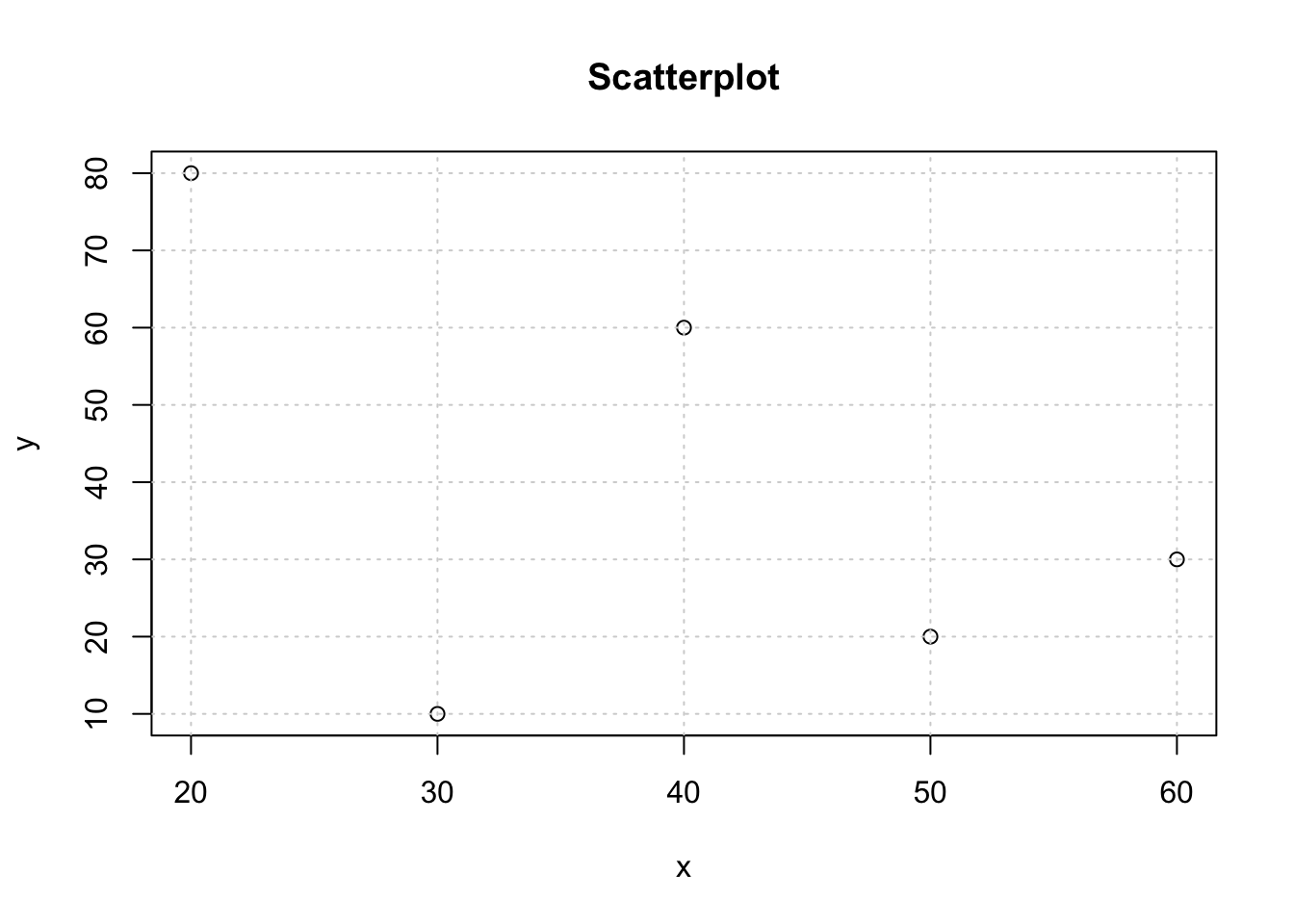
y <-c(80,60,10,20,30)x <-c(20,40,30,50,60)ylab ='y'xlab ='x'plot(x,y,main='Scatterplot',xlab=xlab,ylab=ylab)grid()
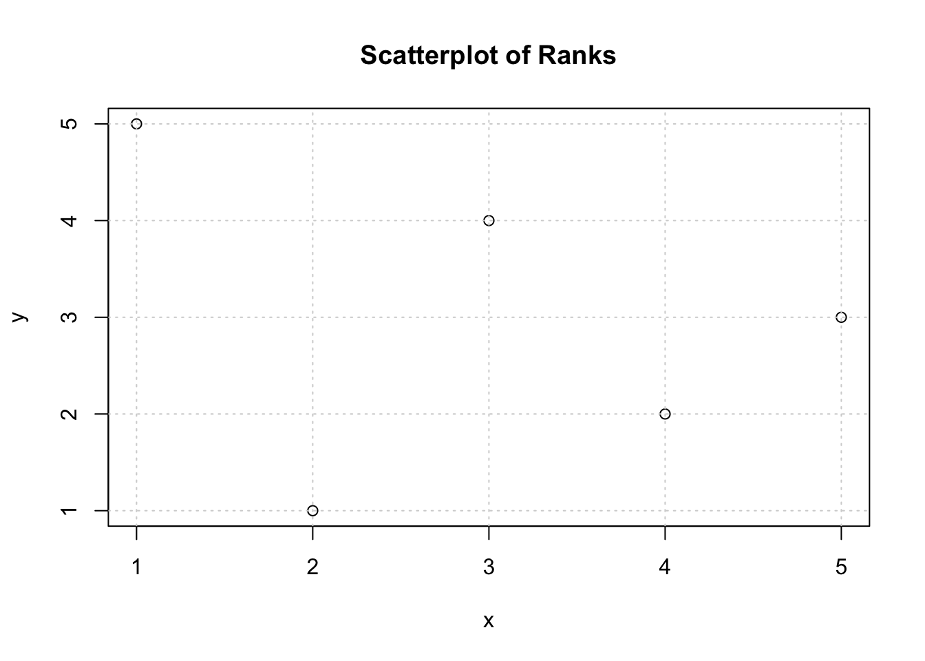
plot(rank(x),rank(y),main='Scatterplot of Ranks',xlab=xlab,ylab=ylab)grid()
#Kendall's tau with base Rk <-cor.test(x,y,method='kendall')#rhok$estimate#2-sided p-valuek$p.value#Spearman's rho with base Rk <-cor.test(x,y,method='spearman')#rhok$estimate#2-sided p-valuek$p.value
 tau
-0.2
[1] 0.8166667
 rho
-0.3
[1] 0.6833333
To compute the Spearman or Kendall \(\tau\) Rank Order Correlation, the R code uses the cor.test function which features a method parameter (method can have the values ‘pearson’, ‘spearman’, and ‘kendall’). Alternatively, there are several external libraries (such as the Kendall package) that can be used.
72.8 Purpose
Rank Order Correlations are used to identify associations between pairs of variables. Since the computations are based on ranks (rather than the original values) they require a hypothesis-testing mechanism (see Hypothesis Testing) which does not rely on distributional assumptions (i.e. Rank Order Correlations are non-parametric).
72.9 Pros & Cons
72.9.1 Pros
Rank Order Correlations have the following advantages:
There are no distributional assumptions when these correlations are used to test hypotheses. In other words, there is no requirement that the variables have a Normal Distribution.
These correlations are robust (not sensitive to outliers).
They are easily computed with many software packages.
72.9.2 Cons
Rank Order Correlations have the following disadvantages:
Some software packages may not correct for ties (software documentation does not always describe whether or not correction for ties is applied, and how this is done)
While most readers know that Rank Order Correlations exist, they often do not know why they are used and how they differ from Pearson Correlations.
72.10 Example 1
The following analysis shows the Spearman Rank Order Correlation for two types of intrinsic motivation scores. Since both variables have a discrete (non normal) distribution, this computation can be used for the purpose of hypothesis testing.
The correlation coefficient is 0.599 which is evidence for a positive association between both types of intrinsic motivation (i.e. students with high scores for IM.Know also tend to have high scores for IM.Accomplishment).
72.11 Example 2
The Kendall \(\tau\) correlation can be computed by selecting “Kendall” in the “Type of Correlations” drop down box. The output show that the correlation is 0.463 which is considerably smaller than the Spearman correlation from the previous example. This is (not always but) often the case: Kendall’s \(\tau\) tends to be more conservative than Spearman’s correlation.
Spearman, Charles. 1904. “The Proof and Measurement of Association Between Two Things.”The American Journal of Psychology 15 (1): 72–101. https://doi.org/10.2307/1412159.