95 Normal Distributions revisited
95.1 Introduction
95.1.1 Case 1
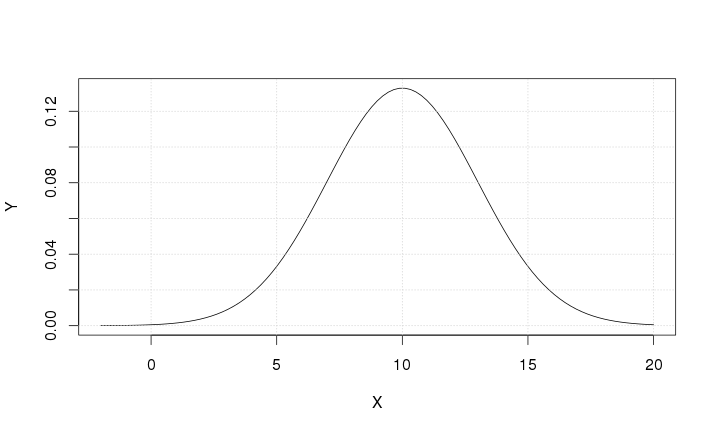
Let us examine the following function
\[ Y=\frac {1}{3\sqrt{\text{2$\pi $}}}e^{-\frac {1} {2} \left(\frac{X-10} {3}\right)^2} \]
95.1.1.1 Solutions & Slopes
It is obvious that \(Y > 0\) because the exponential function is positive (i.e. \(e^x > 0\) for any \(x \in \mathbb{R}\)).
95.1.1.2 Asymptotes
The x-axis is a horizontal asymptote: \(\underset{x \rightarrow \pm \infty }{\text{lim}Y}=0\)
95.1.1.3 Positive & negative slopes
\[ Y' = Y \left( -\frac {1} {2} \right) 2 \left( \frac{X-10} {3} \right) \frac {1} {3} \]
The derivative is positive for \(X < 10\), exactly zero for \(X=10\), and negative for \(X > 10\). The maximum \(\left( Y = \frac {1}{3 \sqrt{2\pi}} \right)\) is reached for \(X=10\).
95.1.1.4 Inflection Points
\[ \begin{matrix} \text{Y"} &=&-\text{cY'}(X-10)-\text{cY} & \\ \text{Y"} &=&-c(X-10)\text{Y'}-\text{cY} & \\ \text{Y"} &=&-c(X-10)\left[-c(X-10)Y\right]-\text{cY} & \\ \text{Y"} &=&\text{cY}\left[c(X-10)^2-1\right] &\text{ where c}=\frac 1 9 \end{matrix} \]
Hence the solutions can be found
\[ \begin{matrix}(X-10)^2=9 \\ X-10=\pm 3 \\ X=7\vee X=13 \end{matrix} \]
There are 2 inflection points: one for \(X=7\) and one for \(X=13\). In both cases the function value is \(Y=\frac{1}{3\sqrt{2\pi}}e^{-\frac{1}{2}} = \frac{1}{3 \sqrt{2\pi e}}\)
95.1.1.5 Chart
95.1.2 Case 2
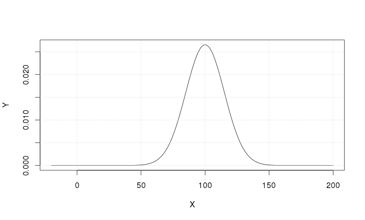
Let us examine the following function
\[ Y=\frac 1{15\sqrt{\text{2$\pi $}}}e^{-\frac 1 2\left(\frac{X-100}{15}\right)^2} \]
95.1.2.1 Solutions & Slopes
\[Y > 0\]
95.1.2.2 Asymptotes
The x-axis: \(\underset{x \rightarrow \pm \infty }{\text{lim}Y}=0\)
95.1.2.3 Positive & negative slopes
\[ \text{Y'}=-\text{cY}(X-100)\text{ where c}=\frac 1{225} \]
The derivative is positive for \(X < 100\), exactly zero for \(X = 100\), and negative for \(X > 100\). The maximum \(\left( Y = \frac{1}{15 \sqrt{2 \pi}} \right)\) is reached for \(X = 100\).
95.1.2.4 Inflection Points
\[ \text{Y'{}'}=\text{cY}\left[c(X-100)^2-1\right] \]
There are inflection points for \(X = 85\) and \(X = 115\).
95.1.2.5 Chart
95.1.3 Case 3
Consider the following function
\[ Y = \frac 1{\sqrt{\mu_2} \sqrt{2 \pi }}e^{- \frac 1 2 \left( \frac{X-\text{E}\left(X\right)}{\sqrt{\mu_2}} \right)^2} \]
95.1.3.1 Task
Based on the previous examples, write down the analysis of this function.
95.1.4 Case 4
Consider the following function
\[Y=\frac 1{\sqrt{\text{2$\pi $}}}e^{-\frac 1 2Z^2}\]
95.1.4.1 Task
Draw the graph of this function.
95.2 Definition of Normal Distribution (revisited)
X is a continuous variable with the following properties:
- the domain is \(\left(-{\infty}, +{\infty}\right)\)
- E\((X) \in \mathbb{R}\)
- \(\mu_2 > 0\):
The variable X is said to be normally distributed with the following density function
\[ Y=\frac 1{\sqrt{\text{2$\pi $}\mu _2}}e^{-\frac 1 2\left[\frac{X-\text{E}(X)}{\sqrt{\mu _2}}\right]^2} \]
if
\[ \forall a \leq b: \text{P}(a \leq X \leq b) = \int_{a}^{b} \frac 1{\sqrt{2 \pi \mu_2}}e^{-\frac 1 2\left[\frac{X-\text{E}(X)}{\sqrt{\mu_2}}\right]^2}\text{d}X \]
where P\((a \leq X \leq b)\) represents the probability of X being included in the interval \([a, b]\).
Since the domain of \(X\) is \(\left(-{\infty}, +{\infty}\right)\) it follows that \(-\infty < X < +\infty\) which implies that P\((-\infty < X < +\infty) = 1\):
\[ \int_{-\infty}^{+\infty} \frac 1{\sqrt{2 \pi \mu_2}}e^{-\frac 1 2\left[\frac{X-\text{E}(X)}{\sqrt{\mu_2}}\right]^2}\text{d}X = 1 \]
95.2.1 Chart of Normal Distribution
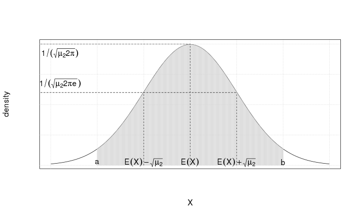
Figure 95.3 shows the chart of the normal density function, including E\((X)\), E\((X) - \sqrt{\mu_2}\), and E\((X) + \sqrt{\mu_2}\):
- E\((X)\) is called the expected value of X (i.e. the mean of X)
- \(\mu_2\) is called the second central moment of X (i.e. the variance of X)
- the shaded area is P\((a \leq X \leq b)\) for any \(a, b \in \mathbb{R}\).
95.2.2 Interpretation of \(\sqrt{\mu_2}\)
The value of \(\sqrt{\mu_2}\) is used to derive central probability intervals of \(X\) -- a few examples are shown here:
\[ \begin{aligned}\text{P} \left( \text{E} \left( X \right) - 0.67 \sqrt{\mu_2} \leq X \leq \text{E} \left( X \right) + 0.67 \sqrt{\mu_2} \right) \simeq 50.00\% \\\text{P} \left( \text{E} \left( X \right) - 1.00 \sqrt{\mu_2} \leq X \leq \text{E} \left( X \right) + 1.00 \sqrt{\mu_2} \right) \simeq 68.26\% \\\text{P} \left( \text{E} \left( X \right) - 1.96 \sqrt{\mu_2} \leq X \leq \text{E} \left( X \right) + 1.96 \sqrt{\mu_2} \right) \simeq 95.00\% \\\text{P} \left( \text{E} \left( X \right) - 2.00 \sqrt{\mu_2} \leq X \leq \text{E} \left( X \right) + 2.00 \sqrt{\mu_2} \right) \simeq 95.44\% \\\text{P} \left( \text{E} \left( X \right) - 3.00 \sqrt{\mu_2} \leq X \leq \text{E} \left( X \right) + 3.00 \sqrt{\mu_2} \right) \simeq 99.74\% \\\text{P} \left( \text{E} \left( X \right) - 3.67 \sqrt{\mu_2} \leq X \leq \text{E} \left( X \right) + 3.67 \sqrt{\mu_2} \right) \simeq 99.98\% \\\text{P} \left( \text{E} \left( X \right) - 4.00 \sqrt{\mu_2} \leq X \leq \text{E} \left( X \right) + 4.00 \sqrt{\mu_2} \right) \simeq 100\%\end{aligned} \]
The last central probability interval seems to contradict the fact that the x-axis is the horizontal asymptote of the Normal Density function which implies that 100% probability is obtained for P\((-\infty \leq X \leq +\infty)\). This apparent contradiction, however, is misleading because
\[ \text{P} \left( \text{E} \left( X \right) - 4.00 \sqrt{\mu_2} \leq X \leq \text{E} \left( X \right) + 4.00 \sqrt{\mu_2} \right) \simeq 99.996\% \]
95.2.3 Standard Normal Table (Gaussian Table)
Consider the problem of finding the probability for
\[\text{P} \left( \text{E} \left( X \right) - 0.6745 \sqrt{\mu_2} \leq X \leq \text{E} \left( X \right) + 0.6745 \sqrt{\mu_2} \right)\]
By definition, this probability can be written as
\[\int_{\text{E}(X) - 0.6745 \sqrt{\mu_2} }^{\text{E}(X) + 0.6745 \sqrt{\mu_2} } \frac 1{\sqrt{2 \pi \mu_2}}e^{-\frac 1 2\left[\frac{X-\text{E}(X)}{\sqrt{\mu_2}}\right]^2}\text{d}X \]
To solve this integral we introduce the following substitution
\[Z = \frac{X - \text{E}(X)}{\sqrt{\mu_2}} \]
which leads to
\[\text{lower bound of } Z = \frac{X - \text{E}(X)}{\sqrt{\mu_2} } = \frac{\text{E}(X) -0.6745\sqrt{\mu_2} - \text{E}(X) }{\sqrt{\mu_2} } = -0.6745\]
and
\[\text{upper bound of } Z = \frac{X - \text{E}(X)}{\sqrt{\mu_2} } = \frac{\text{E}(X) +0.6745\sqrt{\mu_2} - \text{E}(X) }{\sqrt{\mu_2} } = +0.6745\]
and
\[\text{d}Z = \text{d} \frac{X - \text{E}(X) }{\sqrt{\mu_2} } = \frac{1}{\sqrt{\mu_2} } \text{d} \left( X - \text{E}(X) \right) = \frac{1}{\sqrt{\mu_2} } \text{d} X \Rightarrow \text{d} X = \sqrt{\mu_2} \text{d} Z \]
Therefore the integral can be written as
\[\int_{- 0.6745}^{+0.6745} \frac 1{\sqrt{2 \pi}}e^{-\frac 1 2 Z^2}\text{d}Z \]
This is a convenient form because the Gaussian Table (Appendix E) displays
\[\text{P}(0 \leq Z \leq t) = \int_{0}^{t} \frac 1{\sqrt{2 \pi}}e^{-\frac 1 2 Z^2}\text{d}Z\]
which leads to
\[\text{P}(0 \leq Z \leq 0.6745) = \text{P}(-0.6745 \leq Z \leq 0) \simeq 0.25000\]
(note: the normal distribution is symmetric).
Hence, the problem can be solved as follows
\[ P(-0.6745 \leq Z \leq 0.6745) = \int_{- 0.6745}^{+0.6745} \frac 1{\sqrt{2 \pi}}e^{-\frac 1 2 Z^2}\text{d}Z = 2*0.25000 = 0.50000 \; (50.0\%) \]
95.2.4 Corollaries
95.2.4.1 Corollary 1
\[ \begin{aligned}\forall t \geq 0: \text{P} \left( \text{E}(X) - t \sqrt{\mu_2} \leq X \leq \text{E}(X) + t \sqrt{\mu_2} \right) &= \int_{-t}^{t} \frac{1}{\sqrt{2 \pi} } e^{-\frac{1}{2} Z^2} \text{d}Z \\ &= 2 \int_{0}^{t} \frac{1}{\sqrt{2 \pi} } e^{-\frac{1}{2} Z^2} \text{d}Z \end{aligned} \]
This corollary can be used with the Gaussian Table (in Appendix E) to assign probabilities to any value of t:
\[ \begin{aligned}t &=1 & \Rightarrow & 2 * 0.34134 &\simeq 0.68268 &\simeq 68.268\% \\t &=1.96 & \Rightarrow & 2 * 0.47500 &\simeq 0.95000 &\simeq 95.000\% \\t &=2 & \Rightarrow & 2 * 0.47725 &\simeq 0.95450 &\simeq 95.450\% \\t &=3 & \Rightarrow & 2 * 0.49865 &\simeq 0.99730 &\simeq 99.730\%\end{aligned} \]
95.2.4.2 Corollary 2
The variable \(Z\) with probability density \(\frac 1{\sqrt{2 \pi}}e^{-\frac 1 2 Z^2}\text{d}Z\) is normally distributed with E\((Z) = 0\) and \(\mu_2 = 1\).
This is an obvious result because:
\[ \frac 1{\sqrt{2 \pi}}e^{-\frac 1 2 Z^2}\text{d}Z = \frac 1{1 \sqrt{2 \pi}}e^{-\frac 1 2 \left( \frac{Z - 0}{1} \right)^2}\text{d}Z \]
\(Z\) is the so-called Standard Normal Variable which has a Standard Normal (or Gaussian) Distribution.
95.2.4.3 Corollary 3
There are an infinite number of normal distributions because both parameters can vary over their admissible domains: E\((X) \in \mathbb{R}\) and \(\sqrt{\mu_2} \in \mathbb{R}^{+}\).
Here are a few examples:
- \(Y=\frac {1}{3\sqrt{\text{2}\pi}}e^{-\frac {1} {2} \left(\frac{X-10} {3}\right)^2}\) which is the probability density function where E\((X) = 10\) and \(\sqrt{\mu_2} = 3\).
- \(Y=\frac {1}{15\sqrt{\text{2}\pi}}e^{-\frac {1} {2} \left(\frac{X-100} {15}\right)^2}\) which is the probability density function where E\((X) = 100\) and \(\sqrt{\mu_2} = 15\).
- \(Y=\frac {1}{10\sqrt{\text{2}\pi}}e^{-\frac {1} {2} \left(\frac{X-170.5} {10}\right)^2}\) which is the probability density function where E\((X) = 170.5\) and \(\sqrt{\mu_2} = 10\).
- \(Y=\frac {1}{\sqrt{\text{2}\pi}}e^{-\frac {1} {2} Z^2}\) which is the probability density function where E\((X) = 0\) and \(\sqrt{\mu_2} = 1\).
95.2.5 Exercise
Consider the variable X which has a normal distribution with E\((X) = 170.5\) and \(\sqrt{\mu_2} = 10\). What is the probability of X being contained in the interval between 160.5 and 190.5?
The solution is straightforward because the probability density function is
\[Y=\frac {1}{10\sqrt{\text{2$\pi $}}}e^{-\frac {1} {2} \left(\frac{X-170.5} {10}\right)^2}\]
which allows us to write the probability interval as
\[ \text{P}(160.5 \leq X \leq 190.5) = \int\limits_{160.5}^{190.5} \frac {1}{10\sqrt{\text{2$\pi $}}}e^{-\frac {1} {2} \left(\frac{X-170.5} {10}\right)^2}\text{d}X \]
To solve this integral we use the method of substitution
\[Z = \frac{X - 170.5}{10}\]
which allows us to derive the lower bound
\[\frac{160.5 - 170.5}{10} = -1\]
and the upper bound
\[ \frac{190.5 - 170.5}{10} = 2 \]
and
\[\text{d}Z = \text{d} \frac{X - 170.5 }{10 } = \frac{1}{10 } \text{d} \left( X - 170.5 \right) = \frac{1}{10 } \text{d} X \Rightarrow \text{d} X = 10 \text{d} Z \]
Therefore the integral can be written as
\[\int_{- 1}^{+2} \frac 1{\sqrt{2 \pi}}e^{-\frac 1 2 Z^2}\text{d}Z \]
This is a convenient form because the Gaussian Table (Appendix E) displays
\[\text{P}(0 \leq Z \leq t) = \int_{0}^{t} \frac 1{\sqrt{2 \pi}}e^{-\frac 1 2 Z^2}\text{d}Z\]
which leads to
\[\text{P}(0 \leq Z \leq 1) \simeq 0.34134\]
and
\[\text{P}(0 \leq Z \leq 2) \simeq 0.47725\]
Both probabilities should be added to obtain
\[ P(-1 \leq Z \leq 2) \simeq 0.81859 \]
The answer is:
\[ P(160.5 \leq X \leq 190.5) \simeq 81.859\% \]