82 Standard Deviation-Mean Plot

82.1 Definition

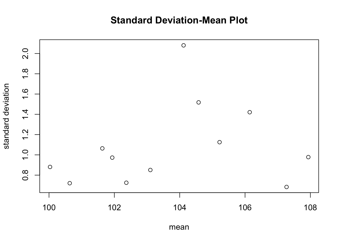
The Standard Deviation-Mean Plot (SMP) consists of a Scatter Plot between the Standard Deviation \(\sigma_i\) versus the Arithmetic Mean \(\mu_i\) for sequential subseries \(i = 1, 2, …, K\). Based on this Scatter Plot, a Simple Linear Regression Model is computed to identify whether or not the Variability (as measured by \(\sigma_i\)) can be explained by (or is associated with) the Central Tendency (as measured by \(\mu_i\)) for each subseries \(i\), i.e.

\[ \sigma_i = \alpha + \beta \mu_i + \epsilon_i \]

where \(K\) is the number of sequential subseries and where the width of each subseries is usually chosen such that each index \(i\) represents one year (assuming we are working with time series which have a seasonal sampling frequency, such as monthly or quarterly series).

If the estimated \(\beta\) coefficient, i.e. \(\hat{\beta}\), is either positive or negative, it can be concluded that the Variability of year \(i\) is associated with the level of that same year -- this is an indication that the Variability can be made more stable by transforming the time series through the Box-Cox transformation (Chapter 71).

82.1.1 Horizontal axis

The Horizontal axis of the SMP displays the Arithmetic Mean of subseries \(i\).

82.1.2 Vertical axis

The vertical axis of the SMP displays the Standard Deviation of subseries \(i\).

82.2 R Module

82.2.1 Public website

The SMP is available on the public website:

https://compute.wessa.net/rwasp_smp.wasp

82.2.2 RFC

The SMP is also available (when using the default profile) in RFC under the “Time Series / Standard Deviation-Mean Plot” menu item.

To compute the Standard Deviation-Mean Plot on your local machine, the following script can be used in the R console:

x <- 100 + cumsum(rnorm(150))
summary(x)
par1 <- 12
n <- length(x)
np <- floor(n / par1)
arr <- array(NA,dim=c(par1,np))
j <- 0
k <- 1
for (i in 1:(np*par1)) {
  j = j + 1
  arr[j,k] <- x[i]
  if (j == par1) {
    j = 0
    k=k+1
  }
}
arr.mean <- array(NA,dim=np)
arr.sd <- array(NA,dim=np)
arr.range <- array(NA,dim=np)
for (j in 1:np) {
  arr.mean[j] <- mean(arr[,j],na.rm=TRUE)
  arr.sd[j] <- sd(arr[,j],na.rm=TRUE)
  arr.range[j] <- max(arr[,j],na.rm=TRUE) - min(arr[,j],na.rm=TRUE)
}
lm1 <- lm(arr.sd~arr.mean)
summary(lm1)
lnlm1 <- lm(log(arr.sd)~log(arr.mean))
summary(lnlm1)
plot(arr.mean,arr.sd,main='Standard Deviation-Mean Plot',xlab='mean',ylab='standard deviation')

plot(arr.mean,arr.range,main='Range-Mean Plot',xlab='mean',ylab='range')

   Min. 1st Qu.  Median    Mean 3rd Qu.    Max. 
  98.88  106.20  108.66  107.87  110.02  115.82 

Call:
lm(formula = arr.sd ~ arr.mean)

Residuals:
    Min      1Q  Median      3Q     Max 
-0.6272 -0.4521 -0.3254  0.1649  1.6413 

Coefficients:
            Estimate Std. Error t value Pr(>|t|)
(Intercept) 11.34866    6.77829   1.674    0.125
arr.mean    -0.09282    0.06266  -1.481    0.169

Residual standard error: 0.7472 on 10 degrees of freedom
Multiple R-squared:   0.18, Adjusted R-squared:  0.09795 
F-statistic: 2.194 on 1 and 10 DF,  p-value: 0.1693


Call:
lm(formula = log(arr.sd) ~ log(arr.mean))

Residuals:
    Min      1Q  Median      3Q     Max 
-0.5829 -0.2888 -0.1663  0.2241  0.8602 

Coefficients:
              Estimate Std. Error t value Pr(>|t|)
(Intercept)     33.878     20.536   1.650    0.130
log(arr.mean)   -7.206      4.385  -1.643    0.131

Residual standard error: 0.4882 on 10 degrees of freedom
Multiple R-squared:  0.2126,    Adjusted R-squared:  0.1339 
F-statistic:   2.7 on 1 and 10 DF,  p-value: 0.1314

To compute the Standard Deviation-Mean Plot, the R code uses the standard lm function to compute the linear regression models that are needed for the SMP analysis.

82.3 Purpose

The SMP is used to identify whether or not the Variability of a time series can be explained by its local level (as measured by the Arithmetic Mean). If the linear relationship \(\sigma_i = \alpha + \beta \mu_i + \epsilon_i\) is confirmed then it may be necessary to transform the time series.

82.4 Pros & Cons

82.4.1 Pros

The SMP has the following advantages:

It is easy to compute and provides useful information about the time series.
It allows the user to derive the parameter of the Box-Cox transformation (this will be explained later).

82.4.2 Cons

The SMP has the following disadvantages:

The SMP cannot be computed with many software packages.
Most readers are not familiar with the SMP.
The SMP is sensitive to outliers (just like the Simple Linear Regression Model).

82.5 Example

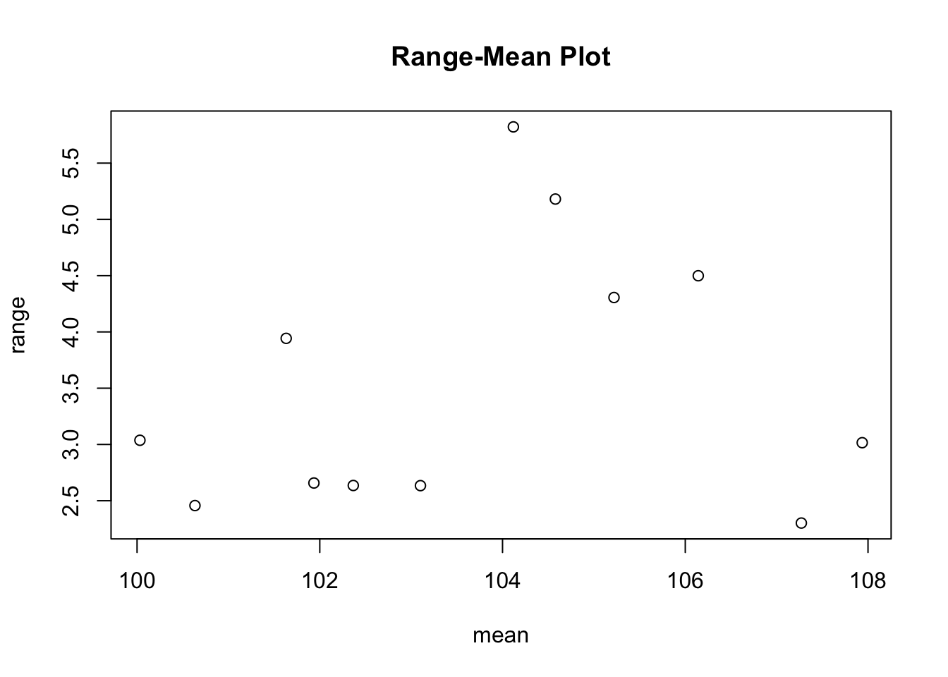
Let us consider the Airline Data and apply the SMP analysis. The following analysis shows for each section (i.e. year) the Arithmetic Mean (column 2), Standard Deviation (column 3), and Range (column 4).

Interactive Shiny app (click to load).

Open in new tab

The corresponding Scatter Plot is also shown. Observe how the dots describe an almost perfect linear relationship between the Standard Deviation \(\sigma_i\) and the Arithmetic Mean \(\mu_i\) of each section \(i\).

The Standard Deviations and Arithmetic Means are used in a Simple Linear Regression Model which allows to estimate the parameters of the regression line that describes the Scatter Plot. The output shows the parameters of the constant term and the slope of the regression line (= 0.1886). This implies that the Standard Deviation (of subsequent years) increases as the Arithmetic Mean increases. Later it will be explained how we can test whether this regression parameter is statistically significant. For now, it is sufficient to know we can (at least) describe the linear relationship between \(\sigma_i\) and \(\mu_i\) based on the SMP.

82.6 Task

Compute the SMP for the monthly Marriages time series and describe your conclusions.