• Descriptive
    • Moments
    • Concentration
    • Central Tendency
    • Variability
    • Stem-and-Leaf Plot
    • Histogram & Frequency Table
    • Data Quality Forensics
    • Conditional EDA
    • Quantiles
    • Kernel Density Estimation
    • Normal QQ Plot
    • Bootstrap Plot

    • Multivariate Descriptive Statistics
  • Distributions
    • Binomial Probabilities
    • Geometric Probabilities
    • Negative Binomial Probabilities
    • Hypergeometric Probabilities
    • Multinomial Probabilities
    • Dirichlet
    • Poisson Probabilities

    • Exponential
    • Gamma
    • Erlang
    • Weibull
    • Rayleigh
    • Maxwell-Boltzmann
    • Lognormal
    • Pareto
    • Inverse Gamma
    • Inverse Chi-Square

    • Beta
    • Power
    • Beta Prime (Inv. Beta)
    • Triangular

    • Normal (area)
    • Logistic
    • Laplace
    • Cauchy (standard)
    • Cauchy (location-scale)
    • Gumbel
    • Fréchet
    • Generalized Extreme Value

    • Normal RNG
    • ML Fitting
    • Tukey Lambda PPCC
    • Box-Cox Normality Plot
    • Noncentral t
    • Noncentral F
    • Sample Correlation r

    • Empirical Tests
  • Hypotheses
    • Theoretical Aspects of Hypothesis Testing
    • Bayesian Inference
    • Minimum Sample Size

    • Empirical Tests
    • Multivariate (pair-wise) Testing
  • Models
    • Manual Model Building
    • Guided Model Building
  • Time Series
    • Time Series Plot
    • Decomposition
    • Exponential Smoothing

    • Blocked Bootstrap Plot
    • Mean Plot
    • (P)ACF
    • VRM
    • Standard Deviation-Mean Plot
    • Spectral Analysis
    • ARIMA

    • Cross Correlation Function
    • Granger Causality
  1. Descriptive Statistics & Exploratory Data Analysis
  2. 78  Probability Plot Correlation Coefficient Plot (PPCC Plot)
  • Preface
  • Getting Started
    • 1  Introduction
    • 2  Why Do We Need Innovative Technology?
    • 3  Basic Definitions
    • 4  The Big Picture: Why We Analyze Data
  • Introduction to Probability
    • 5  Definitions of Probability
    • 6  Jeffreys’ axiom system
    • 7  Bayes’ Theorem
    • 8  Sensitivity and Specificity
    • 9  Naive Bayes Classifier
    • 10  Law of Large Numbers

    • 11  Problems
  • Probability Distributions
    • 12  Bernoulli Distribution
    • 13  Binomial Distribution
    • 14  Geometric Distribution
    • 15  Negative Binomial Distribution
    • 16  Hypergeometric Distribution
    • 17  Multinomial Distribution
    • 18  Poisson Distribution

    • 19  Uniform Distribution (Rectangular Distribution)
    • 20  Normal Distribution (Gaussian Distribution)
    • 21  Gaussian Naive Bayes Classifier
    • 22  Chi Distribution
    • 23  Chi-squared Distribution (1 parameter)
    • 24  Chi-squared Distribution (2 parameters)
    • 25  Student t-Distribution
    • 26  Fisher F-Distribution
    • 27  Exponential Distribution
    • 28  Lognormal Distribution
    • 29  Gamma Distribution
    • 30  Beta Distribution
    • 31  Weibull Distribution
    • 32  Pareto Distribution
    • 33  Inverse Gamma Distribution
    • 34  Rayleigh Distribution
    • 35  Erlang Distribution
    • 36  Logistic Distribution
    • 37  Laplace Distribution
    • 38  Gumbel Distribution
    • 39  Cauchy Distribution
    • 40  Triangular Distribution
    • 41  Power Distribution
    • 42  Beta Prime Distribution
    • 43  Sample Correlation Distribution
    • 44  Dirichlet Distribution
    • 45  Generalized Extreme Value (GEV) Distribution
    • 46  Frechet Distribution
    • 47  Noncentral t Distribution
    • 48  Noncentral F Distribution
    • 49  Inverse Chi-Squared Distribution
    • 50  Maxwell-Boltzmann Distribution
    • 51  Distribution Relationship Map

    • 52  Problems
  • Descriptive Statistics & Exploratory Data Analysis
    • 53  Types of Data
    • 54  Datasheets

    • 55  Frequency Plot (Bar Plot)
    • 56  Frequency Table
    • 57  Contingency Table
    • 58  Binomial Classification Metrics
    • 59  Confusion Matrix
    • 60  ROC Analysis

    • 61  Stem-and-Leaf Plot
    • 62  Histogram
    • 63  Data Quality Forensics
    • 64  Quantiles
    • 65  Central Tendency
    • 66  Variability
    • 67  Skewness & Kurtosis
    • 68  Concentration
    • 69  Notched Boxplot
    • 70  Scatterplot
    • 71  Pearson Correlation
    • 72  Rank Correlation
    • 73  Partial Pearson Correlation
    • 74  Simple Linear Regression
    • 75  Moments
    • 76  Quantile-Quantile Plot (QQ Plot)
    • 77  Normal Probability Plot
    • 78  Probability Plot Correlation Coefficient Plot (PPCC Plot)
    • 79  Box-Cox Normality Plot
    • 80  Kernel Density Estimation
    • 81  Bivariate Kernel Density Plot
    • 82  Conditional EDA: Panel Diagnostics
    • 83  Bootstrap Plot (Central Tendency)
    • 84  Survey Scores Rank Order Comparison
    • 85  Cronbach Alpha

    • 86  Equi-distant Time Series
    • 87  Time Series Plot (Run Sequence Plot)
    • 88  Mean Plot
    • 89  Blocked Bootstrap Plot (Central Tendency)
    • 90  Standard Deviation-Mean Plot
    • 91  Variance Reduction Matrix
    • 92  (Partial) Autocorrelation Function
    • 93  Periodogram & Cumulative Periodogram

    • 94  Problems
  • Hypothesis Testing
    • 95  Normal Distributions revisited
    • 96  The Population
    • 97  The Sample
    • 98  The One-Sided Hypothesis Test
    • 99  The Two-Sided Hypothesis Test
    • 100  When to use a one-sided or two-sided test?
    • 101  What if \(\sigma\) is unknown?
    • 102  The Central Limit Theorem (revisited)
    • 103  Statistical Test of the Population Mean with known Variance
    • 104  Statistical Test of the Population Mean with unknown Variance
    • 105  Statistical Test of the Variance
    • 106  Statistical Test of the Population Proportion
    • 107  Statistical Test of the Standard Deviation \(\sigma\)
    • 108  Statistical Test of the difference between Means -- Independent/Unpaired Samples
    • 109  Statistical Test of the difference between Means -- Dependent/Paired Samples
    • 110  Statistical Test of the difference between Variances -- Independent/Unpaired Samples

    • 111  Hypothesis Testing for Research Purposes
    • 112  Decision Thresholds, Alpha, and Confidence Levels
    • 113  Bayesian Inference for Decision-Making
    • 114  One Sample t-Test
    • 115  Skewness & Kurtosis Tests
    • 116  Paired Two Sample t-Test
    • 117  Wilcoxon Signed-Rank Test
    • 118  Unpaired Two Sample t-Test
    • 119  Unpaired Two Sample Welch Test
    • 120  Two One-Sided Tests (TOST) for Equivalence
    • 121  Mann-Whitney U test (Wilcoxon Rank-Sum Test)
    • 122  Bayesian Two Sample Test
    • 123  Median Test based on Notched Boxplots
    • 124  Chi-Squared Tests for Count Data
    • 125  Kolmogorov-Smirnov Test
    • 126  One Way Analysis of Variance (1-way ANOVA)
    • 127  Kruskal-Wallis Test
    • 128  Two Way Analysis of Variance (2-way ANOVA)
    • 129  Repeated Measures ANOVA
    • 130  Friedman Test
    • 131  Testing Correlations
    • 132  A Note on Causality

    • 133  Problems
  • Regression Models
    • 134  Simple Linear Regression Model (SLRM)
    • 135  Multiple Linear Regression Model (MLRM)
    • 136  Logistic Regression
    • 137  Generalized Linear Models
    • 138  Multinomial and Ordinal Logistic Regression
    • 139  Cox Proportional Hazards Regression
    • 140  Conditional Inference Trees
    • 141  Leaf Diagnostics for Conditional Inference Trees
    • 142  Conditional Random Forests
    • 143  Hypothesis Testing with Linear Regression Models (from a Practical Point of View)

    • 144  Problems
  • Introduction to Time Series Analysis
    • 145  Case: the Market of Health and Personal Care Products
    • 146  Decomposition of Time Series
    • 147  Ad hoc Forecasting of Time Series
  • Box-Jenkins Analysis
    • 148  Introduction to Box-Jenkins Analysis
    • 149  Theoretical Concepts
    • 150  Stationarity
    • 151  Identifying ARMA parameters
    • 152  Estimating ARMA Parameters and Residual Diagnostics
    • 153  Forecasting with ARIMA models
    • 154  Intervention Analysis
    • 155  Cross-Correlation Function
    • 156  Transfer Function Noise Models
    • 157  General-to-Specific Modeling
  • Model Building Strategies
    • 158  Introduction to Model Building Strategies
    • 159  Manual Model Building
    • 160  Model Validation
    • 161  Regularization Methods
    • 162  Hyperparameter Optimization Strategies
    • 163  Guided Model Building in Practice
    • 164  Diagnostics, Revision, and Guided Forecasting
    • 165  Leakage, Target Encoding, and Robust Regression
  • References
  • Appendices
    • Appendices
    • A  Method Selection Guide
    • B  Presentations and Teaching Materials
    • C  R Language Concepts for Statistical Computing
    • D  Matrix Algebra
    • E  Standard Normal Table (Gaussian Table)
    • F  Critical values of Student’s \(t\) distribution with \(\nu\) degrees of freedom
    • G  Upper-tail critical values of the \(\chi^2\)-distribution with \(\nu\) degrees of freedom
    • H  Lower-tail critical values of the \(\chi^2\)-distribution with \(\nu\) degrees of freedom

Table of contents

  • 78.1 Definition
  • 78.2 Horizontal axis
  • 78.3 Vertical axis
  • 78.4 R Module
    • 78.4.1 Public website
    • 78.4.2 RFC
  • 78.5 Purpose
  • 78.6 Pros & Cons
    • 78.6.1 Pros
    • 78.6.2 Cons
  • 78.7 Example
  • 78.8 Task
  1. Descriptive Statistics & Exploratory Data Analysis
  2. 78  Probability Plot Correlation Coefficient Plot (PPCC Plot)

78  Probability Plot Correlation Coefficient Plot (PPCC Plot)

78.1 Definition

The PPCC Plot (Filliben 1975) is generated by an iterative process:

  1. a parameter which defines the shape of a user-specified distribution is set to an initial value
  2. the Probability Plot (i.e. QQ Plot against the specified distribution) is computed for the current value of the shape parameter
  3. the Pearson Correlation coefficient (of the Probability Plot) is computed and stored together with the value of the shape parameter
  4. steps 2 and 3 are repeated until a (pre-specified) final value is reached for the shape parameter
  5. a plot is generated which shows all Pearson Correlation coefficients against their respective shape parameter values

78.2 Horizontal axis

The horizontal axis displays the values of the shape parameter which varied between two pre-specified (minimum and maximum) values.

78.3 Vertical axis

The vertical axis displays the Pearson Correlation coefficients.

78.4 R Module

78.4.1 Public website

The Tukey-Lambda PPCC Plot can be found on the public website:

  • https://compute.wessa.net/rwasp_tukeylambda.wasp

78.4.2 RFC

The Tukey-Lambda PPCC Plot is available in RFC under the “Distributions / Tukey lambda PPCC Plot”.

To compute the Tukey-Lambda PPCC Plot on your local machine, the following script can be used in the R console:
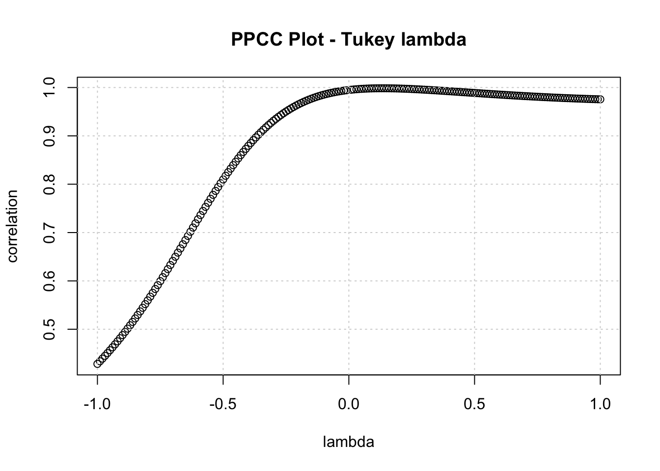
x <- rnorm(500) #should result in lambda = 0.14
#x <- runif(500) #should result in lambda = 1
gp <- function(lambda, p) {
  (p^lambda-(1-p)^lambda)/lambda
}
sortx <- sort(x)
c <- array(NA,dim=c(201))
for (i in 1:201) {
  if (i != 101) c[i] <- cor(gp(ppoints(x), lambda=(i-101)/100),sortx)
}
plot((-100:100)/100,c[1:201],xlab='lambda',ylab='correlation',main='PPCC Plot - Tukey lambda')
grid()

print('Tukey Lambda - Key Values')
cat(paste('\tDistribution (lambda)', 'Correlation\n',
'Approx. Cauchy (lambda=-1)', c[1], '\n',
'Exact Logistic (lambda=0)', (c[100]+c[102])/2, '\n',
'Approx. Normal (lambda=0.14)', c[115], '\n',
'U-shaped Dist. (lambda=0.5)', c[151], '\n',
'Exactly Uniform (lambda=1)', c[201], '\n', sep = '\t'))
[1] "Tukey Lambda - Key Values"
    Distribution (lambda)   Correlation
    Approx. Cauchy (lambda=-1)  0.428325450389276   
    Exact Logistic (lambda=0)   0.994896246857765   
    Approx. Normal (lambda=0.14)    0.998464173639482   
    U-shaped Dist. (lambda=0.5) 0.988786596424759   
    Exactly Uniform (lambda=1)  0.975574929158612   

To compute the Tukey-Lambda PPCC Plot, the R code uses a custom-made function called gp that computes the lambda function. Furthermore, a loop iterates over lambda values between -1 and 1 with a stepsize of 0.01. If a Uniform distribution is used instead of a Normal distribution, the optimal value of lambda changes from 0.14 to 1.

78.5 Purpose

The PPCC Plot is used to find the shape parameter value which produces the best fit (i.e. highest correlation). If the Tukey Lambda PPCC Plot is computed, the value of \(\lambda\) may provide information about the symmetric distribution which fits the data best -- Table 78.1 shows how different values of \(\lambda\) correspond to symmetric distributions.

Warning

The Tukey-Lambda PPCC interpretation table is intended for symmetric distributions only. If the data are clearly skewed, the fitted \(\lambda\) value should not be interpreted as evidence for one of the symmetric families in Table 78.1.

Table 78.1: Tukey-Lambda PPCC Plot for symmetric distributions (source: NIST/SEMATECH (n.d.))
\(\lambda\) Meaning
\(\lambda = -1\) approximate Cauchy distribution
\(\lambda = 0\) distribution is exactly logistic
\(\lambda = 0.14\) distribution is approximately normal
\(\lambda = 0.5\) distribution is reversed U-shaped (i.e. concave)
\(\lambda = 1\) distribution is exactly uniform

78.6 Pros & Cons

78.6.1 Pros

The Tukey-Lambda PPCC Plot has the following advantages:

  • it provides useful information about the distributional shape of the data under investigation
  • it is easy to interpret

78.6.2 Cons

The Tukey-Lambda PPCC Plot has the following disadvantages:

  • there are only few software packages that allow this plot to be generated
  • most readers are not familiar with this plot
  • the plot is not suited for asymmetric distributions

78.7 Example

The following analysis shows the Tukey-Lambda PPCC Plot for the monthly marriages time series in Belgium. From this analysis it can be concluded that the Uniform Distribution has the best fit for the data (see also Table 78.1).

Interactive Shiny app (click to load).
Open in new tab

78.8 Task

Compute the Tukey-Lambda PPCC Plot for the monthly divorces time series and interpret the results. Why does the Divorces time series exhibit a distribution which is completely different from the marriages time series?

Filliben, James J. 1975. “The Probability Plot Correlation Coefficient Test for Normality.” Technometrics 17 (1): 111–17. https://doi.org/10.1080/00401706.1975.10489279.
NIST/SEMATECH. n.d. E-Handbook of Statistical Methods. NIST/SEMATECH. http://www.itl.nist.gov/div898/handbook/.
77  Normal Probability Plot
79  Box-Cox Normality Plot

© 2026 Patrick Wessa. Provided as-is, without warranty.

Feedback: e-mail | Anonymous contributions: click to copy (Sats) | click to copy (XMR)

Cookie Preferences