Poisson modeling answers a common applied question: “how many events occur in a fixed time or space window when events arrive randomly at an average rate?” Examples include call arrivals, defects, accidents, and mutation counts.
Formally, the random variate \(X\) defined for non-negative integers \(X \in \{0, 1, 2, 3, ...\}\) is said to have a Poisson Distribution (i.e. \(X \sim \text{Pois}(\lambda)\)) with rate parameter \(\lambda > 0\).
The Poisson distribution is used to model event counts in fixed intervals when:
Events occur independently of each other
The average rate of occurrence is constant
Two events cannot occur at exactly the same instant
Common applications include:
Number of customers arriving at a service point
Number of defects in a manufactured product
Number of accidents at an intersection
Number of mutations in a DNA sequence
Number of goals scored in a sports match
Number of phone calls received by a call center
The Poisson distribution is also used in Poisson regression (log-linear models) for count data, as an alternative to linear regression when the response variable represents counts. This chapter treats Poisson in more depth because it links directly to multiple approximation results and related-distribution bridges used elsewhere in the handbook.
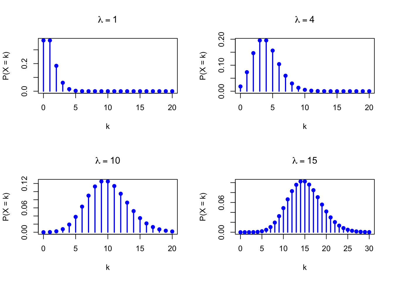
The figure below shows examples of the Poisson Probability Mass Function for different values of \(\lambda\).
Code
par(mfrow =c(2, 2))x <-0:20# Lambda = 1plot(x, dpois(x, lambda =1), type ="h", lwd =2, col ="blue",xlab ="k", ylab ="P(X = k)", main =expression(lambda ==1))points(x, dpois(x, lambda =1), pch =19, col ="blue")# Lambda = 4plot(x, dpois(x, lambda =4), type ="h", lwd =2, col ="blue",xlab ="k", ylab ="P(X = k)", main =expression(lambda ==4))points(x, dpois(x, lambda =4), pch =19, col ="blue")# Lambda = 10plot(x, dpois(x, lambda =10), type ="h", lwd =2, col ="blue",xlab ="k", ylab ="P(X = k)", main =expression(lambda ==10))points(x, dpois(x, lambda =10), pch =19, col ="blue")# Lambda = 15x <-0:30plot(x, dpois(x, lambda =15), type ="h", lwd =2, col ="blue",xlab ="k", ylab ="P(X = k)", main =expression(lambda ==15))points(x, dpois(x, lambda =15), pch =19, col ="blue")par(mfrow =c(1, 1))
Figure 18.1: Poisson Probability Mass Function for various values of lambda
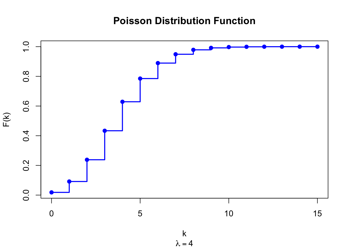
The figure below shows the Poisson Distribution Function for \(\lambda = 4\).
Code
x <-0:15plot(x, ppois(x, lambda =4), type ="s", lwd =2, col ="blue",xlab ="k", ylab ="F(k)", main ="Poisson Distribution Function",sub =expression(lambda ==4))points(x, ppois(x, lambda =4), pch =19, col ="blue")
Figure 18.2: Poisson Distribution Function (lambda = 4)
The equality of mean and variance is a defining characteristic of the Poisson distribution. If the sample variance substantially exceeds the sample mean (overdispersion) or is substantially smaller (underdispersion), the Poisson model may not be appropriate.
18.14 Median
There is no closed-form expression for the median of a Poisson distribution. It can be approximated by
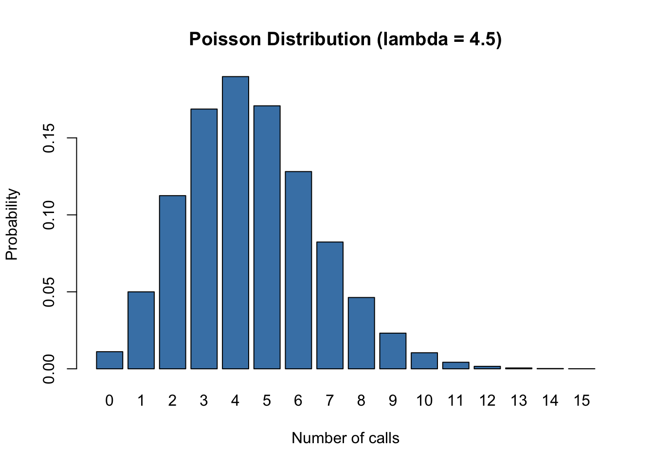
A call center receives an average of 4.5 calls per minute. Assuming calls arrive according to a Poisson process, we can calculate various probabilities:
lambda <-4.5# P(X = 0): probability of no calls in a minutecat("P(no calls):", dpois(0, lambda), "\n")# P(X >= 7): probability of 7 or more callscat("P(7 or more calls):", 1-ppois(6, lambda), "\n")# P(3 <= X <= 6): probability of 3 to 6 callscat("P(3 to 6 calls):", ppois(6, lambda) -ppois(2, lambda), "\n")# Expected number of calls in 5 minutescat("Expected calls in 5 minutes:", 5* lambda, "\n")
P(no calls): 0.011109
P(7 or more calls): 0.1689494
P(3 to 6 calls): 0.6574725
Expected calls in 5 minutes: 22.5
Code
x <-0:15probs <-dpois(x, lambda =4.5)barplot(probs, names.arg = x, col ="steelblue",xlab ="Number of calls", ylab ="Probability",main ="Poisson Distribution (lambda = 4.5)")
Figure 18.3: Poisson distribution for call center example (lambda = 4.5)
18.21 Additional Business Example: Cybersecurity Alert Escalation
A security operations center (SOC) receives an average of \(\lambda = 6.2\) high-priority alerts per hour.
Operations policy requires immediate escalation to an incident commander when 10 or more high-priority alerts arrive in one hour.
This probability quantifies how often the SOC should expect to trigger emergency escalation under current conditions.
If the observed escalation frequency is much higher than this benchmark, it may indicate a changed threat regime (mean rate shift) or alert-quality issues.
This can be integrated into staffing and on-call capacity planning by multiplying the hourly escalation probability by the number of monitored hours per week.
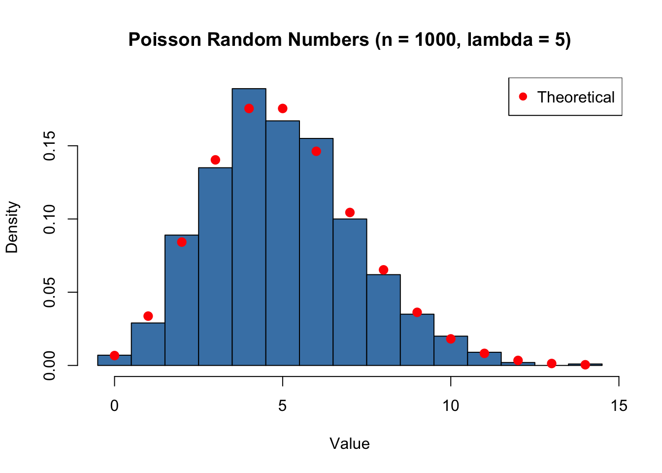
18.22 Random Number Generator
Random numbers from a Poisson distribution can be generated using the rpois function:
18.25 Property 3: Poisson Process Counting Property
If events occur at a constant rate \(\lambda\) per unit time and independently of each other, the number of events in a fixed time interval follows a Poisson distribution. This is known as a Poisson process.
18.26 Property 4: Exponential Interarrival Times
In a Poisson process with rate \(\lambda\), the time between consecutive events follows an Exponential distribution with parameter \(\lambda\).
18.27 Related Distributions 1: Binomial-to-Poisson Limit
The Binomial distribution approaches the Poisson distribution as \(n \rightarrow \infty\) and \(p \rightarrow 0\) while \(np = \lambda\) remains constant:
where \(\lambda = np\). A common rule of thumb is that this approximation is useful when \(n \geq 20\) and \(p \leq 0.05\)(Ross 2014; DeGroot and Schervish 2012).
18.28 Related Distributions 2: Gamma Waiting-Time Relation
The Gamma distribution with shape parameter \(k\) (a positive integer) and rate parameter \(\lambda\) describes the waiting time until the \(k\)-th event in a Poisson process with rate \(\lambda\).
18.29 Related Distributions 3: Conditional Uniform Arrival Times
If \(X \sim \text{Pois}(\lambda)\), then conditionally on \(X=n\), the event times over a fixed interval are distributed as the order statistics of \(n\) i.i.d. Uniform draws on that interval (equivalently: an unordered uniform sample).
Cramér, Harald. 1946. Mathematical Methods of Statistics. Princeton Mathematical Series 9. Princeton: Princeton University Press.
DeGroot, Morris H., and Mark J. Schervish. 2012. Probability and Statistics. 4th ed. Boston: Pearson.
Rao, Calyampudi Radhakrishna. 1945. “Information and the Accuracy Attainable in the Estimation of Statistical Parameters.”Bulletin of the Calcutta Mathematical Society 37: 81–91.
Ross, Sheldon M. 2014. A First Course in Probability. 9th ed. Boston: Pearson.