Cox proportional hazards (Cox PH) regression is used for time-to-event data, also known as survival data. This type of data measures the time until a specific event occurs. Examples include:
Time until death after diagnosis
Time until machine failure
Time until customer churn
Time until first relapse after treatment
Duration of unemployment
A key feature of survival data is censoring: some subjects may not have experienced the event by the end of the study. For these subjects, we know the event did not occur during the observation period, but we do not know when (or if) it will occur. The Cox model handles censored observations naturally.
139.2 Key Concepts
139.2.1 The Survival Function
The survival function \(S(t)\) gives the probability of surviving beyond time \(t\):
\[
S(t) = P(T > t)
\]
where \(T\) is the random variable representing the time to event. \(S(t)\) starts at 1 (everyone alive at the beginning) and decreases over time.
139.2.2 The Hazard Function
The hazard function \(h(t)\) represents the instantaneous rate of the event occurring at time \(t\), given survival up to that point:
\[
h(t) = \lim_{\Delta t \to 0} \frac{P(t \leq T < t + \Delta t \mid T \geq t)}{\Delta t}
\]
The hazard is not a probability – it is a rate and can exceed 1. A higher hazard means a greater instantaneous risk of the event.
139.2.3 Censoring
Table 139.1: Types of censoring
Type
Description
Example
Right censoring
Event has not occurred by end of observation
Patient still alive at study end
Left censoring
Event occurred before observation began
Disease present at first screening
Interval censoring
Event occurred within a known time interval
Infection detected between two clinic visits
The Cox model handles right censoring, the most common type in practice.
139.3 The Cox Proportional Hazards Model
139.3.1 Model Specification
The Cox PH model, proposed by Cox (Cox (1972)), specifies the hazard for individual \(i\) as:
\(h_0(t)\) is the baseline hazard function – the hazard for a subject with all covariates equal to zero
\(\beta_1, ..., \beta_k\) are the regression coefficients
\(X_{i1}, ..., X_{ik}\) are the covariates for subject \(i\)
The model is semi-parametric: the baseline hazard \(h_0(t)\) is left completely unspecified, while the covariate effects are parametric (exponential). This makes the Cox model flexible – it does not assume any particular distribution for survival times.
139.3.2 Interpretation of Coefficients
The coefficients are interpreted as log hazard ratios. Exponentiating gives the hazard ratio (HR):
\[
\text{HR}_j = e^{\beta_j}
\]
The hazard ratio represents the multiplicative change in the hazard for a one-unit increase in \(X_j\), holding other covariates constant:
\(\text{HR} > 1\): the covariate increases the hazard (shorter survival)
\(\text{HR} = 1\): no effect (equivalent to \(\beta_j = 0\))
\(\text{HR} < 1\): the covariate decreases the hazard (longer survival)
For example, if \(\text{HR} = 2\) for a treatment variable (1 = treated, 0 = control), then treated subjects have twice the instantaneous risk of the event at any time point compared to control subjects.
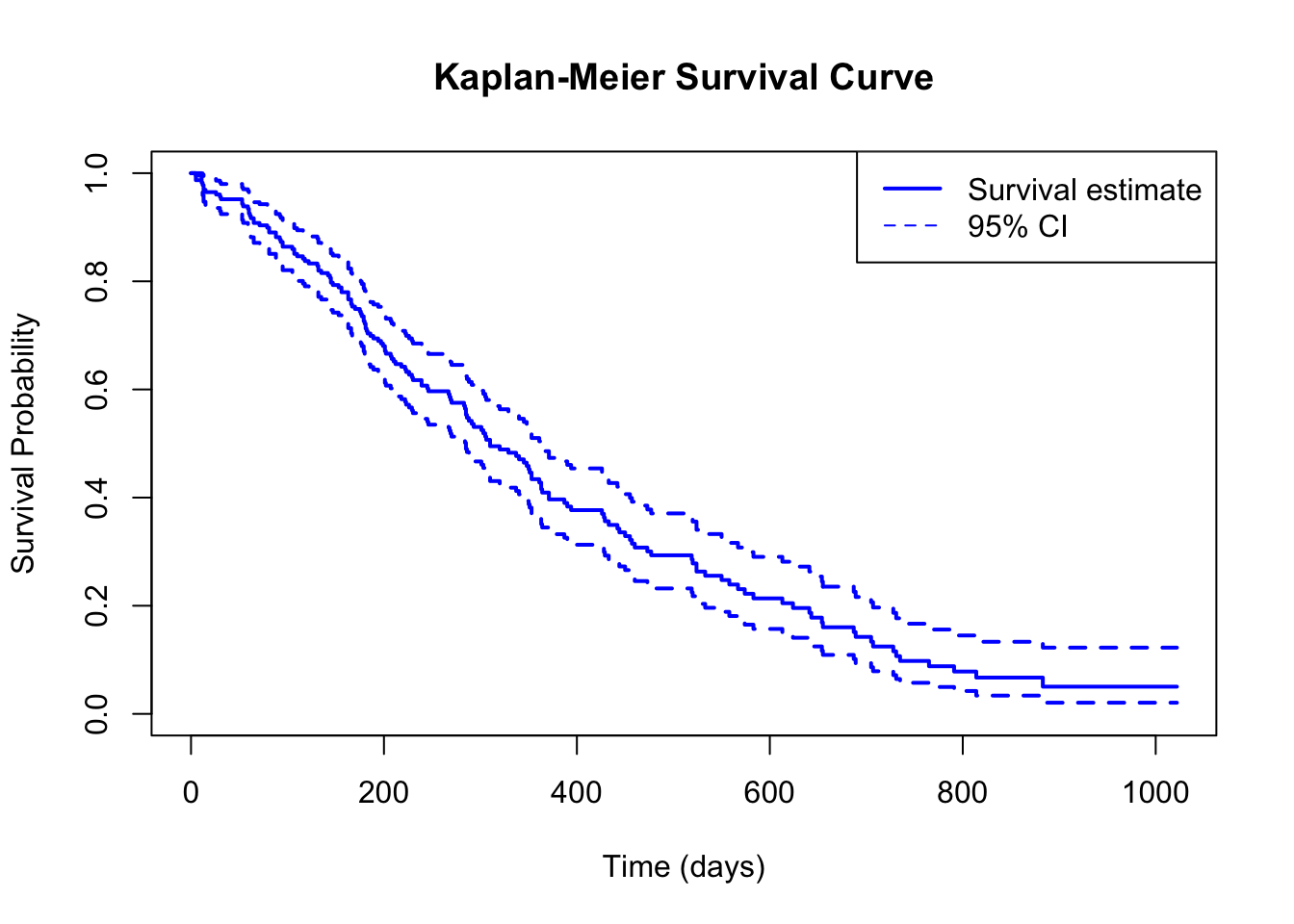
139.4 Kaplan-Meier Curves
Before fitting a Cox model, it is standard practice to visualize survival using Kaplan-Meier curves(Kaplan and Meier 1958) – nonparametric estimates of the survival function.
139.4.1 R Code
library(survival)# Use the lung cancer dataset from the survival package# time: survival time in days# status: 1 = censored, 2 = dead# sex: 1 = male, 2 = femaledata(lung)cat("Dataset overview:\n")cat("n =", nrow(lung), "\n")cat("Events:", sum(lung$status ==2), "\n")cat("Censored:", sum(lung$status ==1), "\n\n")# Kaplan-Meier estimate (overall)km_fit <-survfit(Surv(time, status) ~1, data = lung)cat("Median survival time:", km_fit$table["median"], "days\n")
Dataset overview:
n = 228
Events: 165
Censored: 63

Median survival time: days
From the output above, we can interpret the hazard ratios:
sex (HR < 1 if female = 2): Females have a lower hazard of death, indicating better survival
ph.ecog (physician-rated performance status): Higher ECOG scores indicate worse performance and are associated with higher hazard
age: Each additional year of age is associated with a slight increase in hazard
139.6 Assumptions
139.6.1 Proportional Hazards Assumption
The fundamental assumption of the Cox model is that the hazard ratio between any two subjects is constant over time. In other words, if treatment doubles the hazard at time \(t = 1\), it also doubles the hazard at \(t = 100\).
The baseline hazard \(h_0(t)\) cancels, making the ratio independent of time.
139.6.2 Testing with Schoenfeld Residuals
The proportional hazards assumption can be tested using Schoenfeld residuals (Schoenfeld 1982):
library(survival)data(lung)cox_model <-coxph(Surv(time, status) ~ age + sex + ph.ecog + ph.karno + wt.loss,data = lung)# Test proportional hazards assumptionph_test <-cox.zph(cox_model)print(ph_test)
         chisq df     p
age      0.186  1 0.666
sex      2.059  1 0.151
ph.ecog  1.359  1 0.244
ph.karno 4.916  1 0.027
wt.loss  0.110  1 0.740
GLOBAL   7.174  5 0.208
A significant p-value for a covariate indicates that the proportional hazards assumption may be violated for that variable.
Code
library(survival)data(lung)cox_model <-coxph(Surv(time, status) ~ age + sex + ph.ecog + ph.karno + wt.loss,data = lung)ph_test <-cox.zph(cox_model)# Plot Schoenfeld residuals for each variablepar(mfrow =c(2, 3))for(i in1:5) {plot(ph_test[i], main =names(cox_model$coefficients)[i])}par(mfrow =c(1, 1))
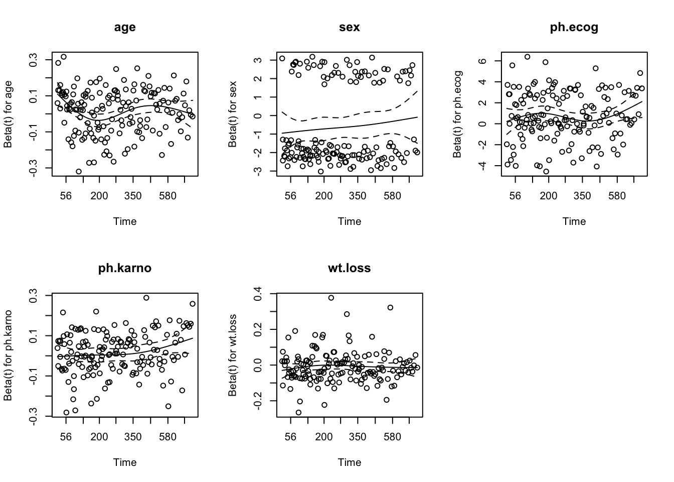
Figure 139.3: Schoenfeld residuals over time for testing proportional hazards
A flat trend in the Schoenfeld residual plot supports the proportional hazards assumption. A clear trend (increasing or decreasing) suggests the effect of that covariate changes over time.
139.6.3 Other Assumptions
Independence of observations: Each subject’s survival is independent of others
Linear relationship between log-hazard and covariates: The effect of each predictor on the log-hazard is linear
Non-informative censoring: The censoring mechanism is unrelated to the probability of the event
139.7 Diagnostics
139.7.1 Martingale Residuals
Martingale residuals are useful for detecting non-linearity in the relationship between a continuous covariate and the log-hazard:
Code
library(survival)data(lung)# Fit null model to get martingale residuals for exploring functional formnull_model <-coxph(Surv(time, status) ~1, data = lung)mart_resid <-residuals(null_model, type ="martingale")# Check functional form for ageplot(lung$age, mart_resid, xlab ="Age", ylab ="Martingale Residuals",main ="Functional Form: Age", pch =20, col =rgb(0, 0, 0, 0.3))lines(lowess(lung$age, mart_resid), col ="red", lwd =2)abline(h =0, lty =2)
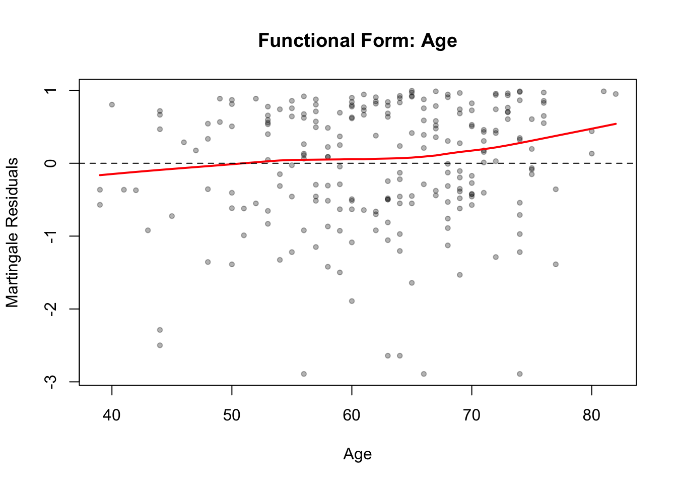
Figure 139.4: Martingale residuals vs. age for checking functional form
A smooth curve close to a straight line supports the linearity assumption. Curvature suggests a transformation or nonlinear term may be needed.
139.7.2 Influence Diagnostics
library(survival)data(lung)cox_model <-coxph(Surv(time, status) ~ age + sex + ph.ecog + ph.karno + wt.loss,data = lung)# dfbeta residuals: influence of each observation on coefficientsdfb <-residuals(cox_model, type ="dfbeta")colnames(dfb) <-names(coef(cox_model))cat("Most influential observations for 'sex' coefficient:\n")top_influence <-order(abs(dfb[, "sex"]), decreasing =TRUE)[1:5]print(data.frame(observation = top_influence,dfbeta_sex =round(dfb[top_influence, "sex"], 4)))
Semi-parametric: no need to specify the distribution of survival times
Handles right-censored data naturally
Coefficients are easily interpretable as hazard ratios
Can accommodate continuous and categorical covariates
Well-established theoretical framework with formal inference
139.8.2 Cons
Requires the proportional hazards assumption (constant hazard ratios over time)
Cannot directly estimate survival probabilities without estimating the baseline hazard
Does not handle time-varying covariates without extensions
Not suitable for recurrent events without modification
Large samples needed for reliable estimation with many covariates
139.9 Task
Using the lung dataset from the survival package, fit a Cox proportional hazards model with at least three predictors. Interpret the hazard ratios and their confidence intervals.
Test the proportional hazards assumption using Schoenfeld residuals. Do any covariates violate the assumption?
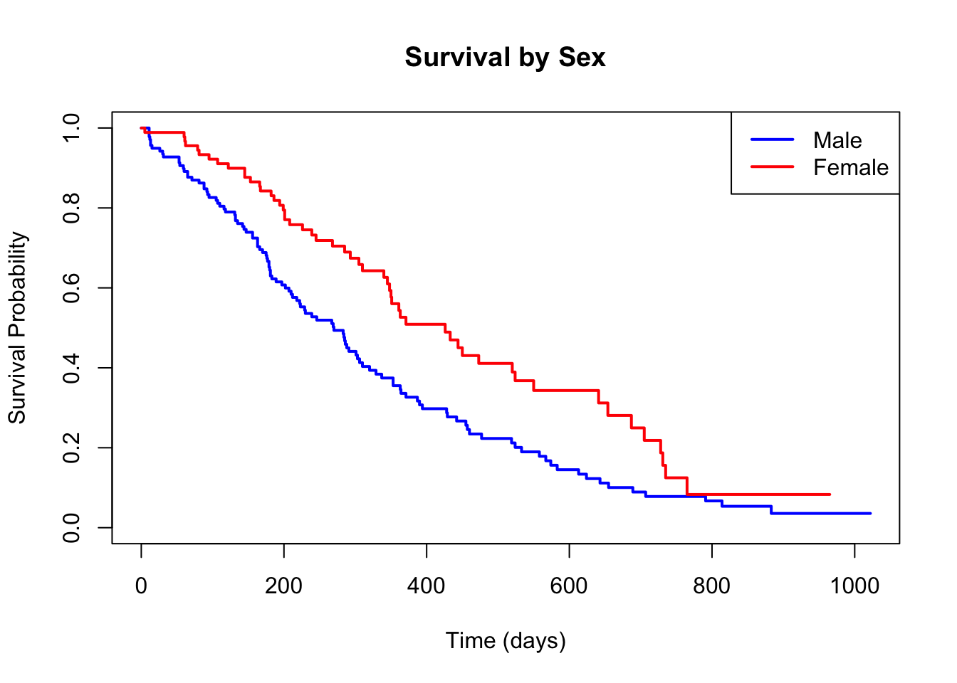
Create Kaplan-Meier curves comparing survival between males and females. Perform a log-rank test and compare the result with the Cox model’s coefficient for sex.
Use martingale residuals to check whether age has a linear relationship with the log-hazard. If not, suggest and fit an appropriate transformation.
Kaplan, Edward L., and Paul Meier. 1958. “Nonparametric Estimation from Incomplete Observations.”Journal of the American Statistical Association 53 (282): 457–81. https://doi.org/10.1080/01621459.1958.10501452.
Mantel, Nathan. 1966. “Evaluation of Survival Data and Two New Rank Order Statistics Arising in Its Consideration.”Cancer Chemotherapy Reports 50 (3): 163–70.
Schoenfeld, David. 1982. “Partial Residuals for the Proportional Hazards Regression Model.”Biometrika 69 (1): 239–41. https://doi.org/10.1093/biomet/69.1.239.