23  Chi-squared Distribution (1 parameter)

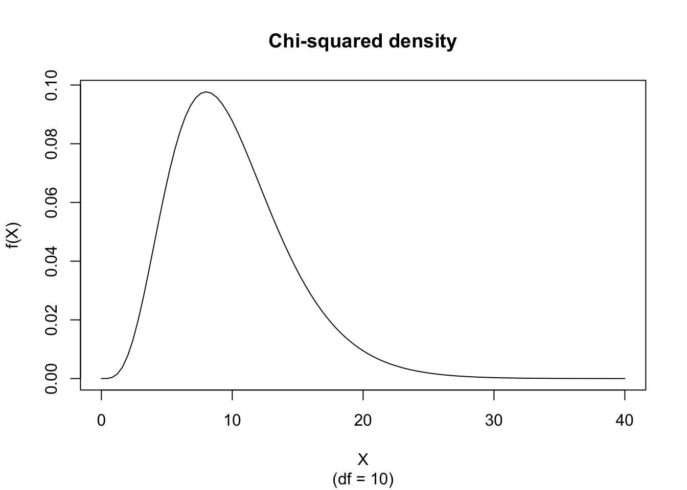
The random variate \(X\) defined for the range \(0 \leq X \leq +\infty\), is said to have a Chi-squared Distribution with 1 parameter (i.e. \(X \sim \chi^2 \left( n \right)\)) with shape parameter \(n \in \mathbb{N}^+\).

23.1 Probability Density Function

\[ \text{f}(X) = \frac{ X^{\frac{n}{2}-1} e^{- \frac{X}{2} } }{ 2^{\frac{n}{2}} \mathrm{ \Gamma} \left[ \frac{n}{2} \right] } \]

The figure below shows an example of the Chi-squared Probability Density function with \(df = 10\).

curve(dchisq(x, df = 10), from = 0, to = 40, xlab="X", ylab="f(X)", main = "Chi-squared density", sub = "(df = 10)")

Figure 23.1: Example of Chi-squared Probability Density Function (df = 10)

23.2 Distribution Function

If \(n/2 \notin \mathbb{N}^+\) then there is no closed form. If \(n/2 \in \mathbb{N}^+\) then

\[ \text{F}(X) = 1 - e^{-\frac{X}{2}} \sum_{j=0}^{r-1} \frac{\left( \frac{X}{2} \right)^j}{j!} \]

where \(r = \frac{n}{2}\).

The figure below shows an example of the Chi-squared Distribution with \(df = 10\).

curve(pchisq(x, df = 10), from = 0, to = 40, xlab="X", ylab="F(X)", main = "Chi-squared distribution", sub = "(df = 10)")

Figure 23.2: Example of Chi-squared Distribution Function (df = 10)

23.3 Moment Generating Function

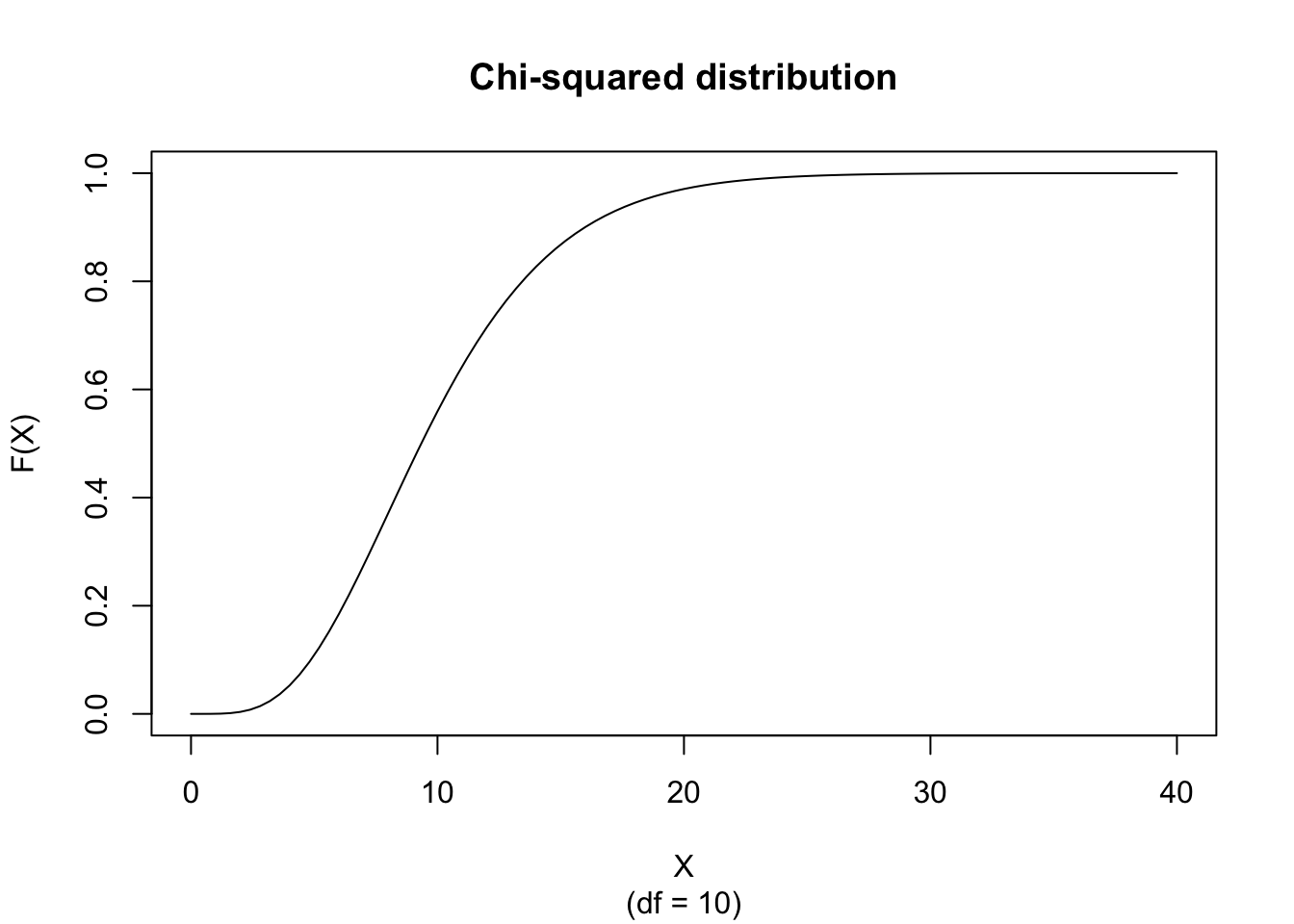
\[ \text{M}_X(t) = (1-2t)^{-\frac{n}{2}} \]

for \(t < \frac{1}{2}\).

23.4 Uncentered Moments

\[ \mu_j' = 2^j \frac{\mathrm{\Gamma}\left[ \frac{n}{2}+j \right]}{\mathrm{\Gamma}\left[ \frac{n}{2} \right]} \]

23.5 Expected Value

\[ \text{E}(X) = n \]

23.6 Variance

\[ \text{V}(X) = 2n \]

23.7 Mode

\[ \text{Mo}(X) = n - 2 \]

for \(n \geq 2\).

23.8 Skewness

\[ g_1 = 2 \sqrt{\frac{2}{n}} \]

23.9 Kurtosis

\[ g_2 = 3 + \frac{12}{n} \]

23.10 Coefficient of Variation

\[ VC = \sqrt{\frac{2}{n}} \]

23.11 R Module

The best fitting Chi-squared Density function can be obtained by estimating the degrees of freedom \(n\) according to the so-called Maximum Likelihood procedure which can be found on the public website:

• https://compute.wessa.net/rwasp_fitdistrchisq1.wasp

The Maximum Likelihood Fitting for the Chi-squared Distribution is also available in RFC under the menu “Distributions / ML Fitting” (you have to select the appropriate function in the designated “Density Function” drop menu).

If you prefer to compute the Chi-squared ML fitting on your local computer, the following code snippets can be used in the R console:

library(MASS)
library(car)
x <- as.numeric(AirPassengers)
chi_df <- fitdistr(x, 'chi-squared', start = list(df=3), method = 'Brent', lower = 0.1, upper = 10000)
chi_k <- chi_df[[1]][1]
cat("estimated df = ", chi_df$estimate, "\n")
cat("standard deviation = ", chi_df$sd, "\n")

estimated df =  256.2321 
standard deviation =  1.882792 

and

xlab <- paste('Chisq(df =', round(chi_df$estimate[[1]],2),')', sep = '')
qqPlot(x, dist = 'chisq', df = chi_df$estimate[[1]], ncp = 0, main = 'QQ plot (Chi-squared 1 param.)', xlab = xlab )

[1] 139 140

Figure 23.3: ML Fitting for Chi-squared Distribution

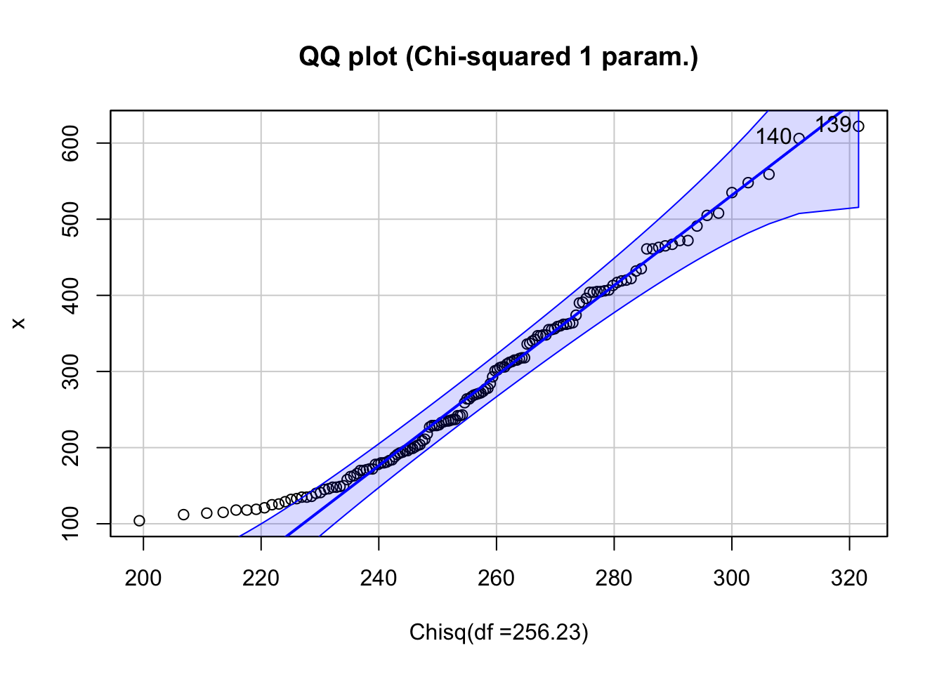
The main function in this R script is fitdistr and is limited by the user-specified lower and upper limit. Instead of displaying a histogram, the script calls the qqPlot function from the car library. The interpretation of this plot is explained in Descriptive Statistics.

23.12 Example

We analyze the time series of monthly divorces (in thousands) and wish to find out whether it can be adequately described by the Chi-squared Distribution. The ML Fitting module can be used to find the best fitting Chi-squared Distribution for the divorces data.

Interactive Shiny app (click to load).

Open in new tab

The estimated degrees of freedom is \(n = 3.46\) but the Chi-squared distribution does not fit the data well (as is shown in the Figure). The visual evidence suggests that a Chi-squared density is not appropriate for these data; for formal goodness-of-fit testing, see Section 2, Section 124.1, and Chapter 125.

23.13 Random Number Generator

If the following is true

\[ \begin{align*} \begin{cases} \text{U}(0,1) \text{ denotes a Uniform Distribution} \\ \text{N}(0,1) \text{ denotes a Standard Normal Distribution} \end{cases} \end{align*} \]

then \(\chi^2(n) \sim -2 \text{ln} \left( \prod_{i=1}^{r} \text{U}_i(0,1) \right)\) with \(r=\frac{n}{2}\) and \(n\) is even

and \(\chi^2(n) \sim -2 \ln \left( \prod_{i=1}^{r} \text{U}_i(0,1) \right) + \left( \text{N}\left( 0, 1 \right) \right)^2\) with \(r=\frac{n-1}{2}\) and \(n\) is odd

23.14 Related Distributions 1: Gamma Representation

The Chi-squared Distribution with one parameter \(n\) is a particular form of the Gamma Distribution. Defined in its general form, the probability density function of the three parameter Gamma Distribution is

\[ \text{f}(Y) = \frac{(Y-c)^{a-1} e^{-\frac{Y-c}{b}}}{\mathrm{\Gamma}[a]b^a} \]

where \(c \leq Y \leq +\infty\), \(0 < a\), \(0 < b\), and \(-\infty \leq c \leq +\infty\).

If the shape parameter \(a = \frac{n}{2}\), the scale parameter \(b = 2\), and the location parameter \(c = 0\), then this three parameter Gamma Distribution is called a Chi-squared Distribution with parameter (degrees of freedom) equal to \(n\).

23.15 Related Distributions 2: Equivalent Gamma Forms

The Chi-squared variate with \(n\) degrees of freedom, is equal to the three parameter Gamma variate with location parameter zero, scale parameter 2, and shape parameter \(n/2\), or equivalently, is twice the Gamma variate with location parameter zero, scale parameter one, and shape parameter \(n/2\).

23.16 Related Distributions 3: Sum of Squares of Standard Normals

The Chi-squared variate with \(n\) degrees of freedom, is equal to the sum of squares of \(n\) independent variates with Standard Normal Distribution, i.e.

\[ \chi^2(n) \sim \sum_{i=1}^{n} Y_i^2 \]

where \(Y_i = \text{N}(0,1)\).

23.17 Related Distributions 4: Large-df Normal Approximation

The Chi-squared variate with degrees of freedom \(n\) (for \(n > 30\)) is approximately equal to half the square of a normal variate with expected value equal to the square root of \((2n-1)\) and unit variance, i.e.

\[ \chi^2(n) \sim \frac{1}{2} Y^2 \]

where \(Y \sim \text{N}(\mu,1)\) with \(\mu = \sqrt{2n-1}\).

23.18 Related Distributions 5: Sum of Squares Around the Population Mean

Given \(n\) independent normal variates with expected value \(\mu\) and variance \(\sigma^2\), the sum of squared deviations from the population mean \(\mu\) is distributed as \(\sigma^2\) times a Chi-squared variate with \(n\) degrees of freedom, i.e.

\[ \frac{ns^2}{\sigma^2} \sim \chi^2(n) \]

or

\[ ns^2 = \sum_{i=1}^{n} \left( x_i - \mu \right)^2 \sim \sigma^2 \chi^2(n) \]

where

\[ s^2 = \frac{1}{n} \sum_{i=1}^{n} \left( x_i - \mu \right)^2 \]

and

\[ X_i \sim \text{N} \left( \mu, \sigma^2 \right) \]

23.19 Related Distributions 6: Sum of Squares Around the Sample Mean

Given \(n\) independent normal variates with expected value \(\mu\) and variance \(\sigma^2\), the sum of squared deviations from the sample mean \(\bar{x}\) is distributed as \(\sigma^2\) times a Chi-squared variate with \(n-1\) degrees of freedom, i.e.

\[ \frac{(n-1)s^2}{\sigma^2} \sim \chi^2(n-1) \]

or

\[ (n-1)s^2 = \sum_{i=1}^{n} \left( x_i - \bar{x} \right)^2 \sim \sigma^2 \chi^2(n-1) \]

where

\[ s^2 = \frac{1}{n-1} \sum_{i=1}^{n} \left( x_i - \bar{x} \right)^2 \]

and

\[ \bar{x} = \frac{1}{n} \sum_{i=1}^{n} x_i \]

and

\[ X_i \sim \text{N} \left( \mu, \sigma^2 \right) \]

23.20 Related Distributions 7: Pooled Chi-squared for Two Samples (Biased Form)

If

\[ \frac{n_1 s_1^2}{\sigma^2} \sim \chi^2 \left( n_1 - 1 \right) \]

\[ \frac{n_2 s_2^2}{\sigma^2} \sim \chi^2 \left( n_2 - 1 \right) \]

then

\[ \frac{n_1 s_1^2 + n_2 s_2^2}{\sigma^2} \sim \chi^2 \left( n_1 + n_2 - 2 \right) \]

where \(s_i^2\) is a biased estimate of \(\sigma^2\), defined as

\[ s_i^2 = \frac{1}{n_i} \sum_{j=1}^{n_i} \left( x_{ij} - \bar{x}_i \right)^2 \]

with

\[ \bar{x}_i = \frac{1}{n_i} \sum_{j=1}^{n_i} x_{ij} \]

and where the observations of sample \(i\) are drawn from a normal population with expected value \(\mu_i\) and variance \(\sigma^2\).

23.21 Related Distributions 8: Ratio of Independent Chi-squared Variables (F)

The Chi-squared variate with \(m\) degrees of freedom, denoted by \(\chi^2(m)\), and the Chi-squared variate with \(n\) degrees of freedom, denoted by \(\chi^2(n)\), are related to the F variate with degrees of freedom \(m\) and \(n\), denoted F\((m,n)\) through the following relationship

\[ \text{F}(m,n) \sim \frac{\frac{\chi^2(m)}{m}}{\frac{\chi^2(n)}{n}} \]

where both Chi-squared variates are independent.

23.22 Related Distributions 9: Chi-squared as a Limit of F

The Chi-squared variate with \(m\) degrees of freedom is equal to \(m\) times the F variate with degrees of freedom \(m\) and \(\infty\), i.e.

\[ \chi^2(m) \sim m \text{F}(m,\infty) \]

23.23 Related Distributions 10: Relation with Student t and Standard Normal

The Chi-squared variate with \(n\) degrees of freedom, denoted by \(\chi^2(n)\), is related to the Student’s t variate with \(n\) degrees of freedom, denoted t\((n)\), and the Standard Normal variate N\((0,1)\) through the following relationship

\[ \chi^2(n) \sim n \frac{\left[\text{N}(0,1)\right]^2}{\left[\text{t}(n)\right]^2} \]

23.24 Related Distributions 11: Link to the Two-parameter Chi-squared Form

The Chi-squared variate \(\chi^2(n)\) can be seen as a special case of the two parameter Chi-squared Distribution \(\chi^2\left( n, \sigma \right)\) with \(\sigma = 1\).

23.25 Related Distributions 12: Poisson Tail Identity

For an even number of degrees of freedom, \(n = 2r\) with \(r \in \mathbb{N}^+\), the Chi-squared variate \(\chi^2(n)\) is related to the Poisson variate with parameter and expected value equal to \(\frac{X}{2}\), denoted by Poi\(\left( \frac{X}{2} \right)\), through

\[ \text{P} \left( \chi^2(2r) \geq X \right) = \text{P} \left( \text{Poi} \left( \frac{X}{2} \right) \leq r - 1 \right) \]

For odd degrees of freedom, compute the tail probability with pchisq() (or the incomplete-gamma form).

23.26 Related Distributions 13: Difference of Two Chi-squared(2) Variables

If \(X\) and \(Y\) are both, independently, Chi-squared variates, each with two degrees of freedom then the variate \(Z = \frac{1}{2} (X - Y)\) follows a double Exponential Distribution, also known as the Laplace Distribution.