The Scatterplot is used to visualise a bivariate dataset (i.e. a dataset containing two variables \(x\) and \(y\)) by plotting each observation as a point on a two dimensional chart. Each point is defined by its coordinates \((x_i,y_i)\) for \(i = 1, 2, 3, …, n\) where \(n\) is the number of observations.
70.2 Horizontal axis
The horizontal axis represents the values for the \(x\) variable.
70.3 Vertical axis
The vertical axis represents the value for the \(y\) variable.
70.4 R Module
The Scatterplot is not available as a separate module but has been integrated into the Correlation module. This is because the Scatterplot is usually used in combination with Correlations and Linear Regression Models.
70.4.1 Public website
The Scatterplot module can be found on the public website:
The Scatterplot module is available in RFC under the menu item “Descriptive / Multivariate Descriptive Statistics”.
If you prefer to compute the Scatterplot on your local machine, the following script can be used in the R console:
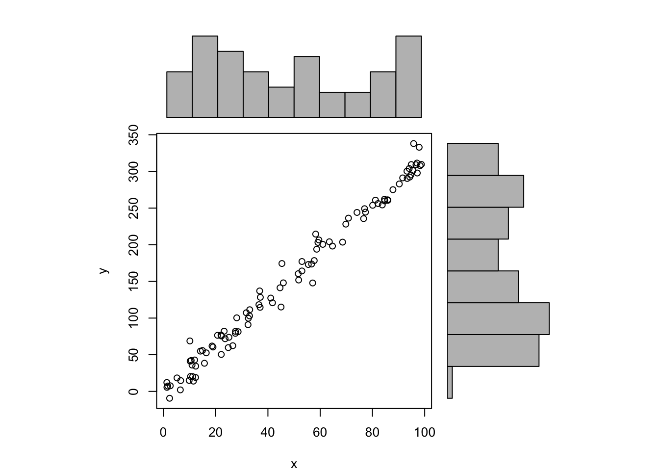
x <-runif(n =100, min =1, max =100)y <-3.2*x +rnorm(n =100, mean =0, sd =12)ylab ='y'xlab ='x'main ='Scatterplot and histograms'histx <-hist(x, plot=FALSE)histy <-hist(y, plot=FALSE)maxcounts <-max(c(histx$counts, histy$counts))xrange <-c(min(x),max(x))yrange <-c(min(y),max(y))nf <-layout(matrix(c(2,0,1,3),2,2,byrow=TRUE), c(3,1), c(1,3), TRUE)par(mar=c(4,4,1,1))plot(x, y, xlim=xrange, ylim=yrange, xlab=xlab, ylab=ylab, sub=main)par(mar=c(0,4,1,1))barplot(histx$counts, axes=FALSE, ylim=c(0, maxcounts), space=0)par(mar=c(4,0,1,1))barplot(histy$counts, axes=FALSE, xlim=c(0, maxcounts), space=0, horiz=TRUE)
cor.test(x, y, method ="pearson")
    Pearson's product-moment correlation

data:  x and y
t = 82.683, df = 98, p-value < 2.2e-16
alternative hypothesis: true correlation is not equal to 0
95 percent confidence interval:
 0.9894605 0.9952316
sample estimates:
      cor
0.9929088
To compute the Scatterplot, the R code uses a combination of a scatterplot (produced by the plot function) and two barplot functions that are used to display the Histogram of both variables under investigation. The script also shows the Pearson Correlation Coefficient and the accompanying Hypothesis Test (see Hypothesis Testing).
70.5 Purpose
The Scatterplot is often used as an exploratory tool -- i.e. to visualize the relationship between two quantitative variables.
70.6 Pros & Cons
70.6.1 Pros
The Scatterplot has the following advantages:
it very easy to compute (even with most spreadsheets)
it is easily understood by most readers
it allows the researcher to identify the shape of the relationship between both variables (e.g. linear versus non-linear)
70.6.2 Cons
The Scatterplot has the following disadvantages:
it is not suited to investigate the relationships between variables with discrete values
it does not always display the true nature of the relationship between both variables
when the number of observations is large, overplotting can obscure the true density of observations; the Bivariate Kernel Density Plot (see Chapter 81) provides a better alternative in such cases
70.7 Example
The scatterplot shown below illustrates the Scatterplot for the US coffee retail prices versus the prices of imported Arabica from Colombia. The Scatterplot has been extended by adding the Histogram of both variables (this is usually not found in Scatterplots).
The Scatterplot seems to suggest that there is a positive relationship between both variables (i.e. US retail prices seem to covary with import prices). The plot also shows that there are certain regions with a high density of points (other regions have a low density).
70.8 Task
In the R module shown above:
click on the Input tab
select AMS in the Stored Data dropdown box
click on the Correlations tab
now select Q1_1 and Q1_2 in the Select Variables box
Now examine the Scatterplot for the two discrete variables and explain the problems that you see.