A conditional random forest is an ensemble of many conditional inference trees. Each tree is fitted on a perturbed version of the training data and is allowed to consider only a random subset of predictors at each split. The final prediction is then obtained by averaging across trees.
For classification, the forest averages class probabilities:
\[
\hat P(Y = c \mid x) = \frac{1}{T}\sum_{t=1}^{T}\hat P_t(Y = c \mid x)
\]
where \(T\) is the number of trees and \(\hat P_t(Y = c \mid x)\) is the class probability from tree \(t\).
For regression, the same idea is used with numeric predictions:
So cforest is not only a classifier. It can also be used as a regression ensemble when the outcome is continuous.
The method belongs to the bagging family of ensemble methods discussed in Section 158.3. In R it is implemented in the party package through cforest().
142.2 From ctree to cforest
The easiest way to understand cforest is to compare it directly with the single-tree method from Chapter 140.
Table 142.1: Single-tree and forest comparison
Aspect
ctree
cforest
Fitted structure
one tree
many conditional inference trees
Main strength
direct interpretation of splits
stronger predictive performance
Main weakness
unstable if the training sample changes
no single diagram to interpret
Typical output
tree plot and leaf summaries
average predictions and variable importance
So the tradeoff is clear:
a single ctree is easier to read,
a single ctree can also be diagnosed leaf by leaf when the outcome is continuous (see Chapter 141),
a cforest is usually harder to explain as a diagram,
but the averaging across many trees often reduces instability and improves out-of-sample prediction.
142.3 Algorithm Intuition
The forest procedure can be read as a four-step loop:
draw a perturbed training sample,
grow one conditional inference tree,
repeat that process many times,
average the resulting predictions.
At each split, the tree does not inspect every predictor. It considers only a random subset. This matters because it prevents one very strong predictor from dominating every tree in exactly the same way, which makes the ensemble more diverse.
The result is a model that is usually less volatile than a single tree, but also less transparent. You can no longer point to one root node and say “this is the whole model.” Instead, you interpret the forest through validation results, prediction behavior, and variable-importance summaries.
142.4 Important Control Parameters
The most important forest settings are the following:
Table 142.2: Main cforest control parameters
Parameter
Meaning
Practical effect
ntree
number of trees in the forest
more trees stabilize the average but take longer to fit
mtry
number of predictors considered at each split
smaller values increase diversity across trees
mincriterion
significance threshold used by the underlying conditional inference trees
higher values make individual trees split more conservatively
minsplit, minbucket
minimum node sizes
prevent very small, unstable leaves
ntree and mtry are hyperparameters in the sense of Section 158.4: they are not estimated automatically from the data and should be chosen with validation rather than by habit.
142.5 R Module
There is currently no separate standalone cforest Shiny app in RFC. Instead, the method is available in two broader applications:
Models / Manual Model Building, where the Tree tab now lets you switch between ctree and cforest,
Models / Guided Model Building, where Conditional forest (cforest) appears as a predictive candidate in tabular workflows.
In the manual app, binary forest classification also exposes a threshold slider. The forest first produces class probabilities. The threshold then converts those probabilities into final class labels, so changing the threshold changes the confusion matrix, sensitivity, specificity, and precision.
Because forest fitting is heavier than fitting a single tree, the embedded manual app uses capped forest settings and may briefly show a waiting message if another forest fit is already running.
The web address still uses the historical path NaiveBayes, but in the menu the application is presented as Models / Manual Model Building.
In this run, the forest outperforms the single tree on both accuracy and AUC. That does not mean the forest is always better. It means the averaging idea is working in this example: the forest is less tied to one particular split structure.
142.7 Classification Thresholds for Binary Forests
Just like a logistic regression or a single binary tree, a binary cforest classifier produces probabilities before it produces final class labels. The threshold determines where those probabilities are converted into Yes and No.
The default threshold of 0.50 is common, but it is not sacred. If false negatives are especially costly, lowering the threshold may be reasonable. If false positives are especially costly, raising it may be better. That is why the manual app includes a threshold slider in the Tree tab for both ctree and cforest.
Changing the threshold changes the binary forest’s classification behavior
Threshold
Accuracy
Sensitivity
Specificity
Precision
0.50
0.794
0.629
0.9
0.800
0.35
0.794
0.786
0.8
0.714
This is the point at which ROC analysis becomes practically useful. The ROC curve tells you how sensitivity and false-positive rate move across thresholds; the threshold table shows what that means for an actual classification rule.
142.8 What the Two Models Look Like
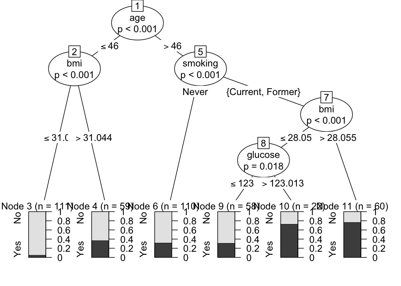
The single tree can still be drawn directly:
Code
plot(disease_tree)
Figure 142.1: Conditional inference tree in the medical example
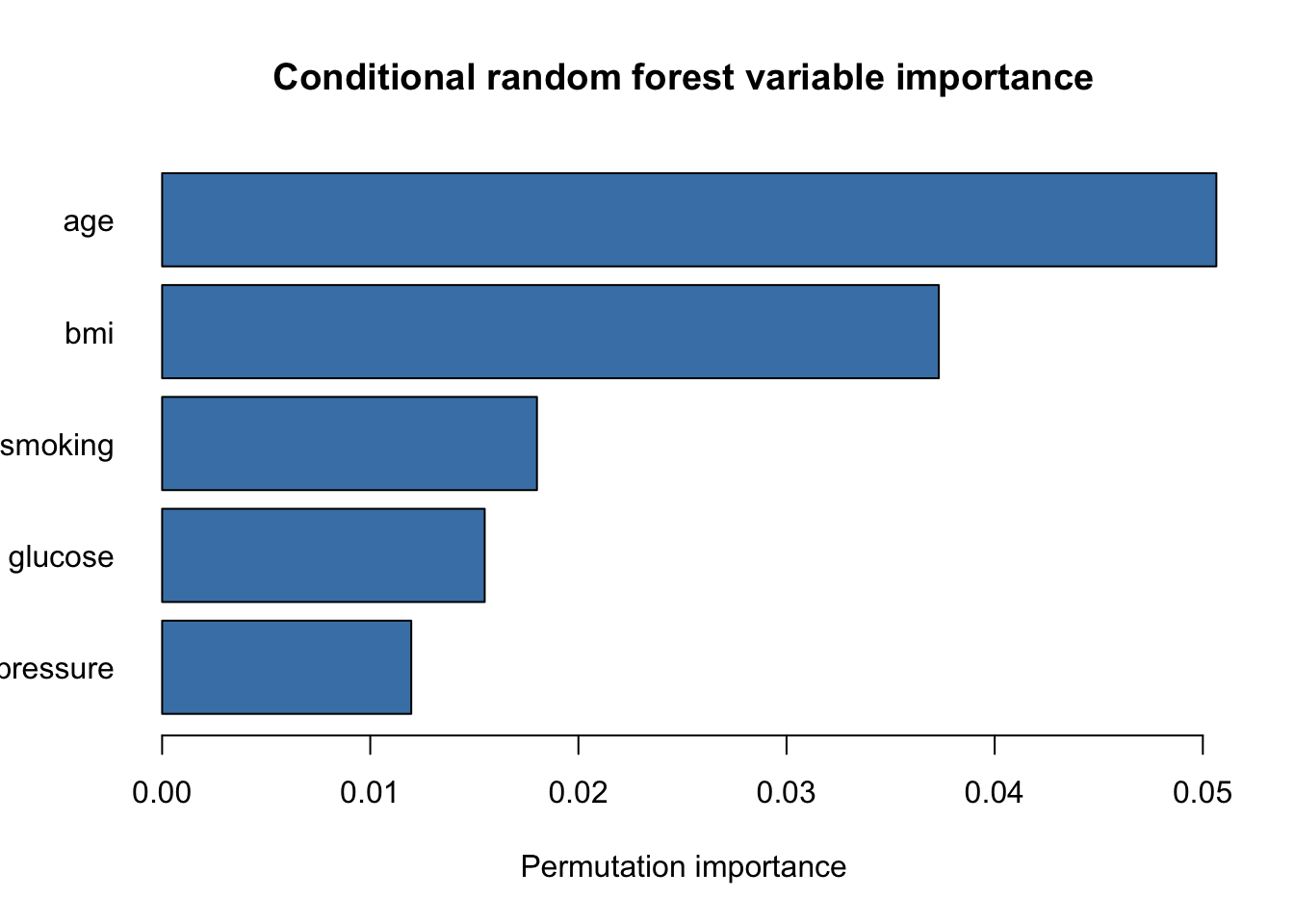
The forest cannot be summarized by one tree diagram. A more appropriate first summary is variable importance:
Figure 142.2: Variable importance from the conditional random forest
This is one of the central interpretive differences:
with ctree, you explain the fitted structure through nodes and splits,
with cforest, you explain the model through predictive performance and variable importance.
That is why cforest is usually a predictive benchmark, not the first explanatory choice.
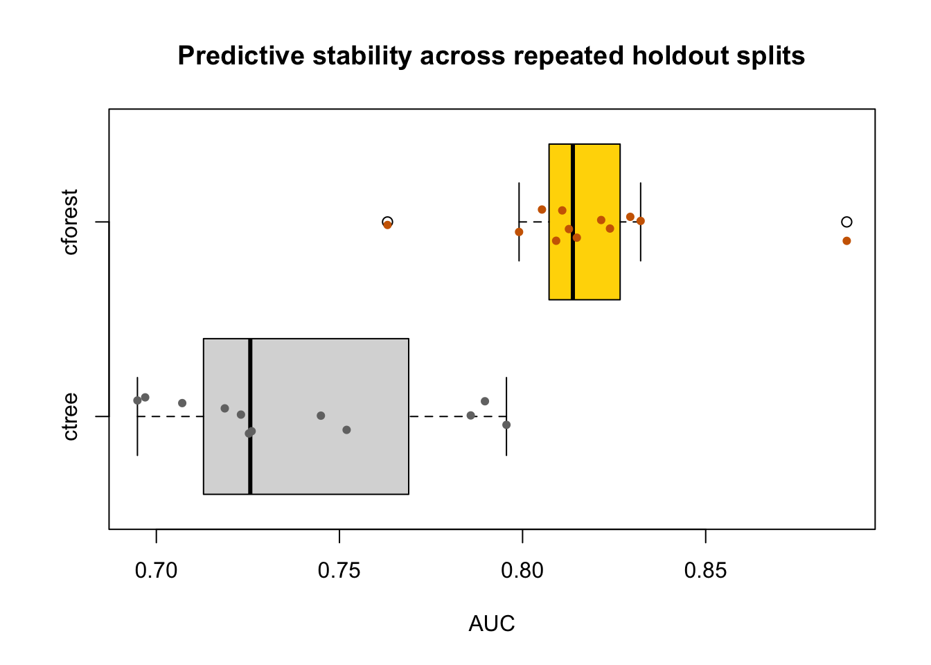
142.9 Repeated Holdout: Average Performance and Reliability
One train/test split is useful, but it does not tell you how stable the comparison is. The next code block therefore repeats the split several times and records the test AUC of both models. This is the same idea introduced formally in Section 160.3.
Figure 142.3: Repeated-holdout AUC distributions for ctree and cforest
This plot should be read exactly the way the guided workflow asks you to read predictive stability:
the box position reflects average predictive quality,
the line inside the box is the median repeated-holdout result,
the spread reflects reliability across splits.
If one model has slightly better average AUC but much wider spread, the final choice becomes a judgment about accuracy versus reliability rather than a purely mechanical ranking.
142.10 How This Connects to the Guided Workflow
The Guided Model Building app does not treat cforest as “just another tree.” It treats it as:
a predictive benchmark against simpler models,
a model whose importance summaries can be inspected,
a model whose repeated-validation stability must be read carefully.
This is why the later chapters on Chapter 163 and Chapter 164 compare forests through validation summaries, stability plots, and revision tables rather than through a single explanatory diagram.
142.11 Pros and Cons
142.11.1 Pros
often stronger predictive performance than a single tree,
less sensitive to one particular training split,
handles nonlinearities and interactions automatically.
142.11.2 Cons
much less directly interpretable than ctree,
slower to fit and diagnose,
variable importance is useful but does not replace a clear model diagram.
142.12 Practical Reading Rule
Use cforest when the goal is mainly prediction and you want a flexible tree-based benchmark. Prefer ctree or logistic regression when the primary goal is explanation and the fitted structure itself must be read directly.
142.13 Task
Recreate the medical example and compare ctree with cforest on a train/test split.
Report both accuracy and AUC. Does the forest improve both?
Inspect the variable-importance plot. Which predictor appears strongest?
Repeat the split several times. Does the model with the higher average AUC also look more stable, or does the comparison involve a tradeoff between performance and reliability?