• Descriptive
    • Moments
    • Concentration
    • Central Tendency
    • Variability
    • Stem-and-Leaf Plot
    • Histogram & Frequency Table
    • Data Quality Forensics
    • Conditional EDA
    • Quantiles
    • Kernel Density Estimation
    • Normal QQ Plot
    • Bootstrap Plot

    • Multivariate Descriptive Statistics
  • Distributions
    • Binomial Probabilities
    • Geometric Probabilities
    • Negative Binomial Probabilities
    • Hypergeometric Probabilities
    • Multinomial Probabilities
    • Dirichlet
    • Poisson Probabilities

    • Exponential
    • Gamma
    • Erlang
    • Weibull
    • Rayleigh
    • Maxwell-Boltzmann
    • Lognormal
    • Pareto
    • Inverse Gamma
    • Inverse Chi-Square

    • Beta
    • Power
    • Beta Prime (Inv. Beta)
    • Triangular

    • Normal (area)
    • Logistic
    • Laplace
    • Cauchy (standard)
    • Cauchy (location-scale)
    • Gumbel
    • Fréchet
    • Generalized Extreme Value

    • Normal RNG
    • ML Fitting
    • Tukey Lambda PPCC
    • Box-Cox Normality Plot
    • Noncentral t
    • Noncentral F
    • Sample Correlation r

    • Empirical Tests
  • Hypotheses
    • Theoretical Aspects of Hypothesis Testing
    • Bayesian Inference
    • Minimum Sample Size

    • Empirical Tests
    • Multivariate (pair-wise) Testing
  • Models
    • Manual Model Building
    • Guided Model Building
  • Time Series
    • Time Series Plot
    • Decomposition
    • Exponential Smoothing

    • Blocked Bootstrap Plot
    • Mean Plot
    • (P)ACF
    • VRM
    • Standard Deviation-Mean Plot
    • Spectral Analysis
    • ARIMA

    • Cross Correlation Function
    • Granger Causality
  1. Box-Jenkins Analysis
  2. 150  Stationarity
  • Preface
  • Getting Started
    • 1  Introduction
    • 2  Why Do We Need Innovative Technology?
    • 3  Basic Definitions
    • 4  The Big Picture: Why We Analyze Data
  • Introduction to Probability
    • 5  Definitions of Probability
    • 6  Jeffreys’ axiom system
    • 7  Bayes’ Theorem
    • 8  Sensitivity and Specificity
    • 9  Naive Bayes Classifier
    • 10  Law of Large Numbers

    • 11  Problems
  • Probability Distributions
    • 12  Bernoulli Distribution
    • 13  Binomial Distribution
    • 14  Geometric Distribution
    • 15  Negative Binomial Distribution
    • 16  Hypergeometric Distribution
    • 17  Multinomial Distribution
    • 18  Poisson Distribution

    • 19  Uniform Distribution (Rectangular Distribution)
    • 20  Normal Distribution (Gaussian Distribution)
    • 21  Gaussian Naive Bayes Classifier
    • 22  Chi Distribution
    • 23  Chi-squared Distribution (1 parameter)
    • 24  Chi-squared Distribution (2 parameters)
    • 25  Student t-Distribution
    • 26  Fisher F-Distribution
    • 27  Exponential Distribution
    • 28  Lognormal Distribution
    • 29  Gamma Distribution
    • 30  Beta Distribution
    • 31  Weibull Distribution
    • 32  Pareto Distribution
    • 33  Inverse Gamma Distribution
    • 34  Rayleigh Distribution
    • 35  Erlang Distribution
    • 36  Logistic Distribution
    • 37  Laplace Distribution
    • 38  Gumbel Distribution
    • 39  Cauchy Distribution
    • 40  Triangular Distribution
    • 41  Power Distribution
    • 42  Beta Prime Distribution
    • 43  Sample Correlation Distribution
    • 44  Dirichlet Distribution
    • 45  Generalized Extreme Value (GEV) Distribution
    • 46  Frechet Distribution
    • 47  Noncentral t Distribution
    • 48  Noncentral F Distribution
    • 49  Inverse Chi-Squared Distribution
    • 50  Maxwell-Boltzmann Distribution
    • 51  Distribution Relationship Map

    • 52  Problems
  • Descriptive Statistics & Exploratory Data Analysis
    • 53  Types of Data
    • 54  Datasheets

    • 55  Frequency Plot (Bar Plot)
    • 56  Frequency Table
    • 57  Contingency Table
    • 58  Binomial Classification Metrics
    • 59  Confusion Matrix
    • 60  ROC Analysis

    • 61  Stem-and-Leaf Plot
    • 62  Histogram
    • 63  Data Quality Forensics
    • 64  Quantiles
    • 65  Central Tendency
    • 66  Variability
    • 67  Skewness & Kurtosis
    • 68  Concentration
    • 69  Notched Boxplot
    • 70  Scatterplot
    • 71  Pearson Correlation
    • 72  Rank Correlation
    • 73  Partial Pearson Correlation
    • 74  Simple Linear Regression
    • 75  Moments
    • 76  Quantile-Quantile Plot (QQ Plot)
    • 77  Normal Probability Plot
    • 78  Probability Plot Correlation Coefficient Plot (PPCC Plot)
    • 79  Box-Cox Normality Plot
    • 80  Kernel Density Estimation
    • 81  Bivariate Kernel Density Plot
    • 82  Conditional EDA: Panel Diagnostics
    • 83  Bootstrap Plot (Central Tendency)
    • 84  Survey Scores Rank Order Comparison
    • 85  Cronbach Alpha

    • 86  Equi-distant Time Series
    • 87  Time Series Plot (Run Sequence Plot)
    • 88  Mean Plot
    • 89  Blocked Bootstrap Plot (Central Tendency)
    • 90  Standard Deviation-Mean Plot
    • 91  Variance Reduction Matrix
    • 92  (Partial) Autocorrelation Function
    • 93  Periodogram & Cumulative Periodogram

    • 94  Problems
  • Hypothesis Testing
    • 95  Normal Distributions revisited
    • 96  The Population
    • 97  The Sample
    • 98  The One-Sided Hypothesis Test
    • 99  The Two-Sided Hypothesis Test
    • 100  When to use a one-sided or two-sided test?
    • 101  What if \(\sigma\) is unknown?
    • 102  The Central Limit Theorem (revisited)
    • 103  Statistical Test of the Population Mean with known Variance
    • 104  Statistical Test of the Population Mean with unknown Variance
    • 105  Statistical Test of the Variance
    • 106  Statistical Test of the Population Proportion
    • 107  Statistical Test of the Standard Deviation \(\sigma\)
    • 108  Statistical Test of the difference between Means -- Independent/Unpaired Samples
    • 109  Statistical Test of the difference between Means -- Dependent/Paired Samples
    • 110  Statistical Test of the difference between Variances -- Independent/Unpaired Samples

    • 111  Hypothesis Testing for Research Purposes
    • 112  Decision Thresholds, Alpha, and Confidence Levels
    • 113  Bayesian Inference for Decision-Making
    • 114  One Sample t-Test
    • 115  Skewness & Kurtosis Tests
    • 116  Paired Two Sample t-Test
    • 117  Wilcoxon Signed-Rank Test
    • 118  Unpaired Two Sample t-Test
    • 119  Unpaired Two Sample Welch Test
    • 120  Two One-Sided Tests (TOST) for Equivalence
    • 121  Mann-Whitney U test (Wilcoxon Rank-Sum Test)
    • 122  Bayesian Two Sample Test
    • 123  Median Test based on Notched Boxplots
    • 124  Chi-Squared Tests for Count Data
    • 125  Kolmogorov-Smirnov Test
    • 126  One Way Analysis of Variance (1-way ANOVA)
    • 127  Kruskal-Wallis Test
    • 128  Two Way Analysis of Variance (2-way ANOVA)
    • 129  Repeated Measures ANOVA
    • 130  Friedman Test
    • 131  Testing Correlations
    • 132  A Note on Causality

    • 133  Problems
  • Regression Models
    • 134  Simple Linear Regression Model (SLRM)
    • 135  Multiple Linear Regression Model (MLRM)
    • 136  Logistic Regression
    • 137  Generalized Linear Models
    • 138  Multinomial and Ordinal Logistic Regression
    • 139  Cox Proportional Hazards Regression
    • 140  Conditional Inference Trees
    • 141  Leaf Diagnostics for Conditional Inference Trees
    • 142  Conditional Random Forests
    • 143  Hypothesis Testing with Linear Regression Models (from a Practical Point of View)

    • 144  Problems
  • Introduction to Time Series Analysis
    • 145  Case: the Market of Health and Personal Care Products
    • 146  Decomposition of Time Series
    • 147  Ad hoc Forecasting of Time Series
  • Box-Jenkins Analysis
    • 148  Introduction to Box-Jenkins Analysis
    • 149  Theoretical Concepts
    • 150  Stationarity
    • 151  Identifying ARMA parameters
    • 152  Estimating ARMA Parameters and Residual Diagnostics
    • 153  Forecasting with ARIMA models
    • 154  Intervention Analysis
    • 155  Cross-Correlation Function
    • 156  Transfer Function Noise Models
    • 157  General-to-Specific Modeling
  • Model Building Strategies
    • 158  Introduction to Model Building Strategies
    • 159  Manual Model Building
    • 160  Model Validation
    • 161  Regularization Methods
    • 162  Hyperparameter Optimization Strategies
    • 163  Guided Model Building in Practice
    • 164  Diagnostics, Revision, and Guided Forecasting
    • 165  Leakage, Target Encoding, and Robust Regression
  • References
  • Appendices
    • Appendices
    • A  Method Selection Guide
    • B  Presentations and Teaching Materials
    • C  R Language Concepts for Statistical Computing
    • D  Matrix Algebra
    • E  Standard Normal Table (Gaussian Table)
    • F  Critical values of Student’s \(t\) distribution with \(\nu\) degrees of freedom
    • G  Upper-tail critical values of the \(\chi^2\)-distribution with \(\nu\) degrees of freedom
    • H  Lower-tail critical values of the \(\chi^2\)-distribution with \(\nu\) degrees of freedom

Table of contents

  • 150.1 Stationarity of the mean
    • 150.1.1 Example: Unemployment
    • 150.1.2 Example: Births
    • 150.1.3 Example: Soldiers
    • 150.1.4 Example: Traffic
    • 150.1.5 Example: Pageviews
  • 150.2 Stationarity of the variance
    • 150.2.1 Transformation of time series
    • 150.2.2 Standard Deviation-Mean Plot (revisited)
    • 150.2.3 Box-Cox Normality Plot
    • 150.2.4 Example: Unemployment
    • 150.2.5 Example: Births
    • 150.2.6 Example: Soldiers
    • 150.2.7 Example: Traffic
    • 150.2.8 Example: Pageviews
  • 150.3 Why do we need stationarity?
  1. Box-Jenkins Analysis
  2. 150  Stationarity

150  Stationarity

In a first step we need to induce stationarity in the mean and the variance of the time series under investigation. In practice, most time series do not satisfy the stationarity conditions which are required to apply univariate forecasting models. Therefore, these times series are called non-stationary and should be differenced and transformed such that they become stationary with respect to the variance and the mean.

150.1 Stationarity of the mean

With the use of the Autocorrelation Function (ACF) it is possible to detect non-stationarity of the time series with respect to the mean level. As an alternative, it is possible to use the Cumulative Periodogram (CP) to identify non-stationarity. A third diagnostic tool is the so-called Variance Reduction Matrix (VRM) which lists the variances of the time series after several combinations of non-seasonal and seasonal differencing have been applied. As a general rule, the optimal degree of differencing induces stationarity in the mean with a minimum variance.

Stationarity of the mean can be induced by using the backshift and differencing operators. The backshift operator introduces time lags as is illustrated in the following examples:

  • \(B Y_t = Y_{t-1}\)
  • \(B^k Y_t = Y_{t-k}\)
  • \(B_s Y_t = Y_{t-s}\)
  • \(B^k_s Y_t = Y_{t-k s}\)

The differencing operator is called nabla and transforms the time series in terms of past changes:

  • \(\nabla Y_t = (1 - B) Y_t = Y_t - Y_{t-1}\)
  • \(\nabla^2 Y_t = (1 - B) (1 - B) Y_t = (1 - B) (Y_t - Y_{t-1}) \\ = Y_t - Y_{t-1} - Y_{t-1} + Y_{t-2} = Y_t - 2 Y_{t-1} + Y_{t-2}\)
  • \(\nabla_s Y_t = (1 - B_s) Y_t = Y_t - Y_{t-s}\)
  • \(\nabla \nabla_s Y_t = (1 - B) (Y_t - Y_{t-s}) = Y_t - Y_{t-1} - Y_{t-s} + Y_{t-s-1}\)

In practice, we apply the following differencing operators to induce stationarity in the mean:

\(\nabla^d \nabla^D_s Y_t = W_t\)

where

  • \(Y_t\) is the original (raw) time series
  • \(d\) is the degree or order of non-seasonal differencing
  • \(D\) is the degree or order of seasonal differencing
  • \(s\) is the seasonal period
  • \(W_t\) represents the stationary (working) time series

Differencing can be applied to remove non-seasonal and/or seasonal trends. This procedure works reasonably well for a wide range of time series that are naturally observed. Hence, there are only two parameters that need to be determined to induce stationarity in the mean in most commonly encountered time series: the degree of non-seasonal differencing \(d\) and the degree of seasonal differencing \(D\).

As a general rule, we can detect a non-seasonal stochastic trend (unit-root-type behavior) in the ACF if the sequence of the first \(s/2\) autocorrelations exhibits a slowly decreasing pattern. The degree of non-seasonal differencing \(d\) is increased by one unit as long as this pattern is observed. In most cases, the pattern will disappear after a single round of non-seasonal differencing has been applied (i.e. \(d=1\)).

We can detect a seasonal trend in the ACF if the sequence of autocorrelations at lags \({s, 2s, 3s}\) exhibits a slowly decreasing pattern. The degree of seasonal differencing \(D\) is increased by one unit as long as this pattern is observed. In most cases, the pattern will disappear after a single round of seasonal differencing has been applied (i.e. \(D=1\)).

In practice, we will often encounter time series that can be made stationary in the mean through differencing with \(d \in {0, 1, 2}\) and \(D \in {0,1}\).

In addition, we can use the CP to identify seasonal and non-seasonal trend components whenever the CP line exhibits large (step-wise) increases which correspond to the long term or seasonal periods.

150.1.1 Example: Unemployment

The Unemployment time series should be differenced with the non-seasonal differencing operator because the ACF is slowly decreasing, as is shown in the output:

Interactive Shiny app (click to load).
Open in new tab

Hence, we set the slider to \(d=1\) (degree of non-seasonal

differencing = 1) and recompute the ACF. The result indicates that the time series also contains a seasonal trend (observe how the ACF at seasonal time lags is slowly decreasing).

Therefore, we must set \(d=D=1\) (\(D\) is the degree of seasonal differencing) by moving the seasonal differencing slider and recompute the ACF.

The ACF (with \(d=D=1\)) suggests that the time series \(\nabla \nabla_{12} Y_t\) is stationary in the mean. This will be verified through spectral analysis in order to gain more confidence in the degrees of non-seasonal and seasonal differencing.

Interactive Shiny app (click to load).
Open in new tab

The output shows the CP of the original time series and indicates a non-seasonal stochastic trend because the CP value increases sharply at the frequency of the longest period (i.e. on the left side of the chart).

If we apply non-seasonal differencing (\(d=1\)) then the CP indicates the presence of a seasonal trend. The CP (with \(d=D=1\) and \(s=12\)) suggests that the time series \(\nabla \nabla_{12} Y_t\) is stationary in the mean.

Finally, we examine the VRM (Variance Reduction Matrix) with seasonal period \(s = 12\). The analysis confirms the above findings because the lowest (trimmed) variance can be found for \(d=D=1\):

Interactive Shiny app (click to load).
Open in new tab

150.1.2 Example: Births

We examine the following computations to find the appropriate values for d and D:

Interactive Shiny app (click to load).
Open in new tab
Interactive Shiny app (click to load).
Open in new tab
Interactive Shiny app (click to load).
Open in new tab

The ACF and CP seem to suggest \(D=0\) and \(d=0\) (even though there could be doubt about \(d=1\)). The VRM, however, suggests \(D=1\) and \(d=0\). There seems to be a discrepancy between the three diagnostic tools. Therefore, we formulate three alternative models:

  • Model 1: \(Y_t\)
  • Model 2: \(\nabla Y_t\)
  • Model 3: \(\nabla_{12} Y_t\)

150.1.3 Example: Soldiers

We examine the following computations to find the appropriate values for d and D:

Interactive Shiny app (click to load).
Open in new tab
Interactive Shiny app (click to load).
Open in new tab
Interactive Shiny app (click to load).
Open in new tab

All three diagnostics suggest that \(D=0\) and \(d=1\). Therefore we can conclude that \(\nabla Y_t\) is stationary in the mean.

150.1.4 Example: Traffic

The examination of the Traffic data can be obtained in a similar way. Hint: this time series has no seasonality. Therefore, it is not possible to find any seasonal effects.

The ACF and VRM suggest that \(D=0\) and \(d=1\). Based on the CP we may doubt whether \(d=1\) is appropriate or not. Therefore, we formulate two alternative models:

  • Model 1: \(Y_t\)
  • Model 2: \(\nabla Y_t\)

150.1.5 Example: Pageviews

The examination of the Pageviews data can be obtained in a similar way. Note: the pageviews time series has a daily sampling frequency. Therefore we should use s=7 instead of s=121.

150.2 Stationarity of the variance

150.2.1 Transformation of time series

If we write a time series \(Y_t\) as the sum of a deterministic mean and a disturbance term

\[ Y_t = \mu_t + e_t \]

then the relationship between V\((Y_t)\) and \(\mu_t\) may be of the form

\[ \text{V}(Y_t) = \sigma^2 h^2(\mu_t) \]

where \(h\) is an arbitrary function.

The time series \(Y_t\) must therefore be transformed in order to stabilize the variance. Denote the transformed series by \(g(Y_t)\) and expand it using a Taylor series around \(\mu_t\)

\[ g(Y_t) \simeq g(\mu_t) + (Y_t - \mu_t)g'(\mu_t) \]

This can be used to obtain the variance of the transformed series

\[ \begin{aligned} \text{V}(g( Y_t )) &\simeq \text{V}\left( g(\mu_t) + (Y_t - \mu_t) g'(\mu_t) \right) \\ &\simeq \left( g'(\mu_t) \right)^2 \text{V}(Y_t)\\ &\simeq \left( g'(\mu_t) \right)^2 h^2(\mu_t) \sigma^2 \end{aligned} \]

which implies that the variance can be stabilized by imposing

\[ g'(\mu_t) = \frac{1}{h(\mu_t)} \]

Accordingly, if the standard deviation of the series is proportional to the mean level (\(\sigma_{Y_t} \propto \mu_t\)) then

\[ h(\mu_t) = \mu_t \Rightarrow g'(\mu_t) = \frac{1}{\mu_t} \]

from which it follows that

\[ g(\mu_t) = \ln \mu_t \]

In case the variance of the time series is proportional to the mean level then

\[ h(\mu_t) = \sqrt{\mu_t} \Rightarrow g'(\mu_t) = \frac{1}{\sqrt{\mu_t}} \]

from which it follows that

\[ g(\mu_t) = 2 \sqrt{\mu_t} \]

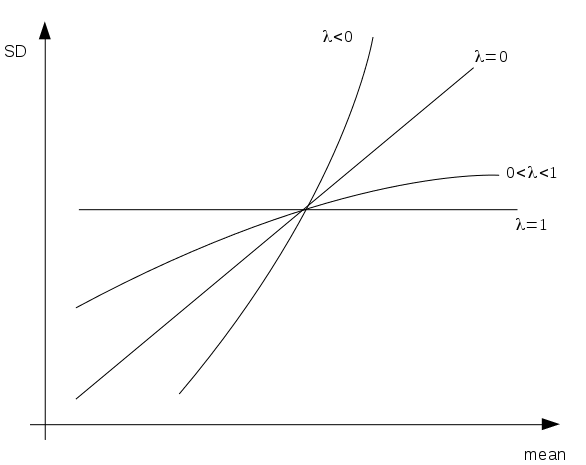
In the Standard Deviation-Mean Plot, the functional relationship is assumed to be as follows

\[ \sigma_{Y_t} = \alpha \mu_{Y_t}^{1-\lambda} \]

The value of \(\lambda\) is the parameter of the so-called “simple” Box-Cox transformation (Box and Cox 1964)

\[ \begin{cases}Y_t^\lambda \text{ for } \lambda \neq 0 \\\ln Y_t \text{ for } \lambda = 0\end{cases} \]

Depending on the type of relationship between the Arithmetic Mean and Standard Deviation a different value of \(\lambda\) will be chosen as is shown in Figure 150.1.

Figure 150.1: Theoretical SMP patterns

150.2.2 Standard Deviation-Mean Plot (revisited)

We examine the relationship between the mean and the standard deviation of the time series in order to detect a common form of heteroskedasticity which can be easily removed by the use of a (simplified) Box–Cox transform that is defined as follows: \(Y_t^{\lambda}\) for \(\lambda \neq 0\) and \(\ln Y_t\) for \(\lambda = 0\).

The Standard Deviation-Mean Plot allows us to identify whether a transformation is necessary and it also provides an estimate for \(\lambda\). Note: it is not always possible to find appropriate values for \(\lambda\). In addition, there is no guarantee that the Box-Cox transform allows us to induce stationarity of the Variance. There are many other types of transformation and analysis that might be useful in this respect -- these, however, are beyond the scope of this book.

Formally, the SMP computes two Simple Linear Regression Models based on the Standard Deviation and Arithmetic Mean of sequential blocks. The first model is

\[ \sigma_i = \alpha + \beta \mu_i + \epsilon_i \]

for \(i = 1, 2, …, k\), where \(\sigma_i\) is the Standard Deviation, \(\mu_i\) is the Arithmetic Mean, and \(k\) is the number of sequential blocks. In most cases, we use a “block width” which is equal to the seasonal period \(s\) (e.g. \(s=12\) for monthly time series).

The Hypothesis Test which is used to decide whether a Box-Cox transformation is required, is formulated as follows

\[ \begin{cases}\text{H}_0: \beta = 0 \\\text{H}_A: \beta \neq 0\end{cases} \]

unless we have prior knowledge about the relationship between \(\sigma_i\) and \(\mu_i\).

If we reject the Null Hypothesis then we decide that a Box-Cox transformation is required, i.e. \(\lambda \neq 1\).

The second Simple Linear Regression Model is only required if the Null Hypothesis H\(_0: \beta = 0\) is rejected. It can be shown that the (quasi-)optimal value for \(\lambda\) can be obtained as follows:

\[ \lambda = 1 - \beta \]

where \(\beta\) is obtained through

\[ \ln \sigma_i = \alpha + \beta \ln \mu_i + \epsilon_i \]

which (implicitly) assumes that \(\forall i = 1, 2, …,k: \mu_i > 0\). If any local mean \(\mu_i \leq 0\) then we simply add a constant \(c\) to all observations such that no negative local means remain.

150.2.3 Box-Cox Normality Plot

150.2.3.1 Definition

As an alternative for the SMP it is sometimes useful to employ the Box-Cox Normality Plot which attempts to estimate the (quasi-)optimal value of \(\lambda\) based on the so-called Maximum Likelihood Estimation procedure.

The Box-Cox Normality Plot features two flavors of the Box-Cox transformation: the so-called “full” version and the “simplified” version.

150.2.3.1.1 Full Box-Cox Transformation

The full Box-Cox transformation is defined as follows

\[ \begin{cases}\frac{sign(Y_t)|Y_t|^\lambda-1}{\lambda} \text{ for } \lambda \neq 0 \\\ln Y_t \text{ for } \lambda = 0\end{cases} \]

which is the default setting for the Box-Cox Normality Plot.

150.2.3.1.2 Simple Box-Cox Transformation

The simplified Box-Cox transformation has already been defined in the SMP procedure.

150.2.3.2 Horizontal axis

The horizontal axis of the Box-Cox Normality Plot shows the values of \(\lambda\).

150.2.3.3 Vertical axis

The vertical axis of the Box-Cox Normality Plot shows the correlation of the Normal QQ Plot.

150.2.3.4 R Module

The Box-Cox Normality Plot is available on the public website:

  • https://compute.wessa.net/rwasp_boxcoxnorm.wasp

The same R module is also available (when using the default profile) in RFC under the “`Distributions / Box-Cox Normality Plot” menu item.

If you prefer to compute the Box-Cox Normality Plot on your local machine, the following script can be used in the R console:

library(car)
x <- AirPassengers
par1 = 'Full Box-Cox transform' #Type of transformation
par2 = -2 #Minimum lambda
par3 = 2 #Maximum lambda
par4 = 0 #Constant term to be added before analysis is performed
par5 = 'No' #Display table with original and transformed data
par2 <- abs(par2*100)
par3 <- par3*100
numlam <- par2 + par3 + 1
x <- x + par4
n <- length(x)
c <- array(NA,dim=c(numlam))
l <- array(NA,dim=c(numlam))
mx <- -1
mxli <- -999
for (i in 1:numlam) {
  l[i] <- (i-par2-1)/100
  if (l[i] != 0)
  {
    if (par1 == 'Full Box-Cox transform') x1 <- (x^l[i] - 1) / l[i]
    if (par1 == 'Simple Box-Cox transform') x1 <- x^l[i]
  } else {
    x1 <- log(x)
  }
  c[i] <- cor(qnorm(ppoints(x), mean=0, sd=1),sort(x1))
  if (mx < c[i]) {
    mx <- c[i]
    mxli <- l[i]
    x1.best <- x1
  }
}
print(c) #correlations
print(mx) #maximum correlation
print(mxli) #lambda value of maximum correlation
print(x1.best)
if (mxli != 0) {
  if (par1 == 'Full Box-Cox transform') x1 <- (x^mxli - 1) / mxli
  if (par1 == 'Simple Box-Cox transform') x1 <- x^mxli
} else {
  x1 <- log(x)
}
#Maximum Likelihood approach to find optimal lambda
mypT <- powerTransform(x)
summary(mypT)
plot(l,c,main='Box-Cox Normality Plot', xlab='Lambda',ylab='correlation')
mtext(paste('Optimal Lambda =',mxli))
grid()

hist(x,main='Histogram of Original Data',xlab='X',ylab='frequency')
grid()

hist(x1,main='Histogram of Transformed Data', xlab='X',ylab='frequency')
grid()

qqPlot(x)
grid()
mtext('Original Data')

qqPlot(x1)
grid()
mtext('Transformed Data')

  [1] 0.9102139 0.9107995 0.9113842 0.9119681 0.9125511 0.9131331 0.9137143
  [8] 0.9142945 0.9148737 0.9154520 0.9160293 0.9166056 0.9171809 0.9177552
 [15] 0.9183284 0.9189006 0.9194717 0.9200416 0.9206105 0.9211783 0.9217449
 [22] 0.9223103 0.9228746 0.9234376 0.9239995 0.9245601 0.9251195 0.9256776
 [29] 0.9262345 0.9267900 0.9273443 0.9278972 0.9284487 0.9289990 0.9295478
 [36] 0.9300952 0.9306412 0.9311858 0.9317289 0.9322706 0.9328108 0.9333495
 [43] 0.9338866 0.9344223 0.9349563 0.9354888 0.9360197 0.9365490 0.9370767
 [50] 0.9376027 0.9381271 0.9386498 0.9391708 0.9396901 0.9402076 0.9407234
 [57] 0.9412375 0.9417497 0.9422601 0.9427688 0.9432755 0.9437804 0.9442835
 [64] 0.9447846 0.9452839 0.9457812 0.9462765 0.9467699 0.9472613 0.9477507
 [71] 0.9482380 0.9487234 0.9492066 0.9496878 0.9501669 0.9506439 0.9511187
 [78] 0.9515914 0.9520620 0.9525303 0.9529965 0.9534604 0.9539220 0.9543815
 [85] 0.9548386 0.9552934 0.9557460 0.9561962 0.9566440 0.9570895 0.9575326
 [92] 0.9579733 0.9584115 0.9588474 0.9592807 0.9597116 0.9601400 0.9605659
 [99] 0.9609893 0.9614101 0.9618283 0.9622440 0.9626571 0.9630675 0.9634753
[106] 0.9638805 0.9642830 0.9646828 0.9650799 0.9654743 0.9658659 0.9662548
[113] 0.9666409 0.9670243 0.9674048 0.9677825 0.9681573 0.9685293 0.9688984
[120] 0.9692647 0.9696280 0.9699884 0.9703458 0.9707004 0.9710519 0.9714004
[127] 0.9717460 0.9720885 0.9724280 0.9727644 0.9730977 0.9734280 0.9737552
[134] 0.9740793 0.9744002 0.9747180 0.9750326 0.9753440 0.9756523 0.9759574
[141] 0.9762592 0.9765578 0.9768531 0.9771452 0.9774340 0.9777195 0.9780018
[148] 0.9782806 0.9785562 0.9788284 0.9790972 0.9793627 0.9796248 0.9798835
[155] 0.9801387 0.9803906 0.9806390 0.9808839 0.9811254 0.9813634 0.9815979
[162] 0.9818289 0.9820564 0.9822803 0.9825008 0.9827176 0.9829309 0.9831407
[169] 0.9833468 0.9835494 0.9837483 0.9839437 0.9841354 0.9843234 0.9845078
[176] 0.9846886 0.9848657 0.9850391 0.9852088 0.9853748 0.9855371 0.9856957
[183] 0.9858505 0.9860017 0.9861491 0.9862927 0.9864325 0.9865686 0.9867009
[190] 0.9868295 0.9869542 0.9870751 0.9871922 0.9873055 0.9874150 0.9875207
[197] 0.9876225 0.9877204 0.9878145 0.9879048 0.9879912 0.9880737 0.9881523
[204] 0.9882271 0.9882979 0.9883649 0.9884280 0.9884871 0.9885424 0.9885937
[211] 0.9886412 0.9886847 0.9887242 0.9887599 0.9887916 0.9888194 0.9888432
[218] 0.9888631 0.9888790 0.9888910 0.9888991 0.9889031 0.9889033 0.9888994
[225] 0.9888916 0.9888798 0.9888641 0.9888444 0.9888207 0.9887931 0.9887615
[232] 0.9887259 0.9886863 0.9886428 0.9885953 0.9885438 0.9884883 0.9884289
[239] 0.9883654 0.9882981 0.9882267 0.9881514 0.9880721 0.9879888 0.9879015
[246] 0.9878103 0.9877151 0.9876160 0.9875129 0.9874058 0.9872948 0.9871798
[253] 0.9870609 0.9869380 0.9868112 0.9866804 0.9865457 0.9864071 0.9862645
[260] 0.9861180 0.9859676 0.9858132 0.9856550 0.9854928 0.9853267 0.9851568
[267] 0.9849829 0.9848051 0.9846234 0.9844379 0.9842485 0.9840552 0.9838581
[274] 0.9836571 0.9834522 0.9832435 0.9830310 0.9828146 0.9825944 0.9823704
[281] 0.9821426 0.9819109 0.9816755 0.9814363 0.9811933 0.9809465 0.9806960
[288] 0.9804417 0.9801837 0.9799219 0.9796564 0.9793872 0.9791142 0.9788376
[295] 0.9785572 0.9782732 0.9779855 0.9776941 0.9773990 0.9771003 0.9767980
[302] 0.9764920 0.9761825 0.9758693 0.9755525 0.9752321 0.9749081 0.9745806
[309] 0.9742495 0.9739149 0.9735768 0.9732351 0.9728899 0.9725412 0.9721890
[316] 0.9718333 0.9714742 0.9711116 0.9707456 0.9703761 0.9700032 0.9696270
[323] 0.9692473 0.9688642 0.9684778 0.9680880 0.9676949 0.9672984 0.9668987
[330] 0.9664956 0.9660892 0.9656795 0.9652666 0.9648504 0.9644310 0.9640084
[337] 0.9635825 0.9631535 0.9627213 0.9622858 0.9618473 0.9614056 0.9609607
[344] 0.9605128 0.9600617 0.9596076 0.9591504 0.9586901 0.9582268 0.9577604
[351] 0.9572911 0.9568187 0.9563434 0.9558651 0.9553838 0.9548996 0.9544124
[358] 0.9539224 0.9534294 0.9529336 0.9524349 0.9519333 0.9514290 0.9509217
[365] 0.9504117 0.9498989 0.9493834 0.9488650 0.9483439 0.9478201 0.9472936
[372] 0.9467644 0.9462325 0.9456979 0.9451607 0.9446209 0.9440784 0.9435334
[379] 0.9429857 0.9424355 0.9418827 0.9413274 0.9407695 0.9402092 0.9396463
[386] 0.9390810 0.9385133 0.9379430 0.9373704 0.9367953 0.9362179 0.9356381
[393] 0.9350559 0.9344713 0.9338845 0.9332953 0.9327038 0.9321101 0.9315140
[400] 0.9309158 0.9303153
[1] 0.9889033
[1] 0.22
           Jan       Feb       Mar       Apr       May       Jun       Jul
1949  8.289824  8.438033  8.762263  8.695127  8.509943  8.828220  9.101473
1950  8.364682  8.626761  8.956776  8.828220  8.603691  9.121706  9.523962
1951  9.040128  9.141833  9.667021  9.394411  9.560211  9.667021 10.020032
1952  9.542128  9.702000  9.922260  9.719376  9.753904 10.315193 10.491415
1953  9.971438  9.971438 10.576849 10.562729 10.477008 10.674407 10.954491
1954 10.099767  9.838955 10.562729 10.448045 10.548562 10.954491 11.419910
1955 10.660605 10.534347 10.993071 11.018603 11.031313 11.568630 12.089424
1956 11.205517 11.119274 11.591083 11.546066 11.602268 12.188904 12.558098
1957 11.568630 11.408265 12.008293 11.925727 11.998052 12.639408 13.010198
1958 11.841667 11.602268 12.069272 11.925727 12.079359 12.754500 13.221592
1959 12.049034 11.862826 12.493896 12.400665 12.621457 13.068001 13.656123
1960 12.594405 12.353359 12.612456 12.976862 13.068001 13.560238 14.170466
           Aug       Sep       Oct       Nov       Dec
1949  9.101473  8.849951  8.462160  8.082257  8.438033
1950  9.523962  9.299192  8.784378  8.339900  8.935650
1951 10.020032  9.771058  9.375552  9.060686  9.450454
1952 10.660605 10.177993  9.889142  9.560211  9.938718
1953 11.056625 10.590923 10.208874  9.702000 10.052112
1954 11.313998 10.889426 10.477008 10.083943 10.477008
1955 11.915302 11.534741 11.081791 10.590923 11.131698
1956 12.484654 11.998052 11.466193 11.043987 11.466193
1957 13.026782 12.475394 11.915302 11.454667 11.799058
1958 13.331825 12.475394 12.038882 11.512007 11.809747
1959 13.735881 12.993558 12.503121 12.069272 12.484654
1960 14.063471 13.355135 12.976862 12.343841 12.728181
bcPower Transformation to Normality 
  Est Power Rounded Pwr Wald Lwr Bnd Wald Upr Bnd
x     0.148           0      -0.2374       0.5335

Likelihood ratio test that transformation parameter is equal to 0
 (log transformation)
                            LRT df    pval
LR test, lambda = (0) 0.5662479  1 0.45175

Likelihood ratio test that no transformation is needed
                           LRT df       pval
LR test, lambda = (1) 18.62702  1 1.5895e-05
[1] 139 140
[1] 139 140

150.2.3.5 Example

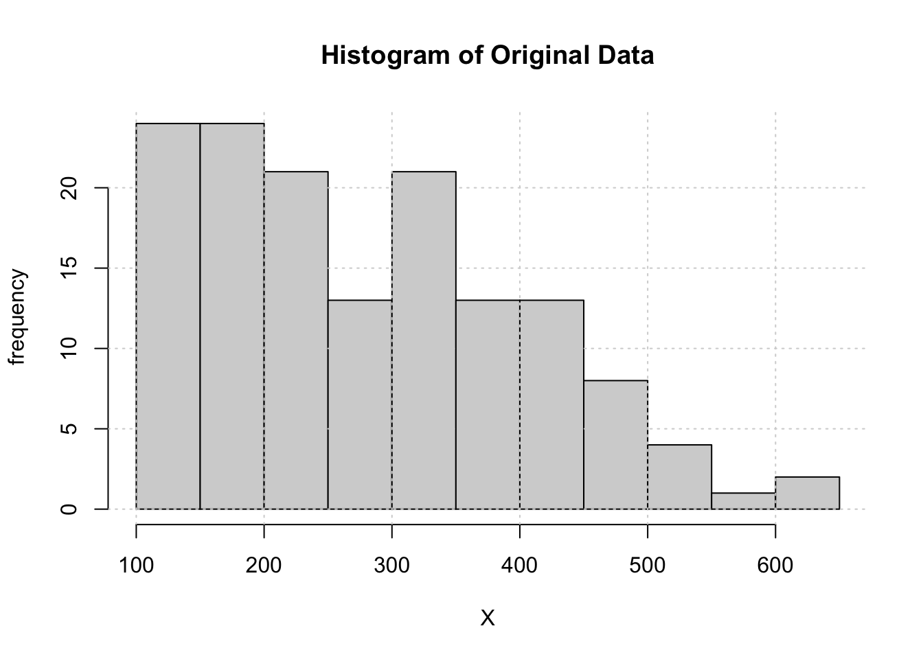
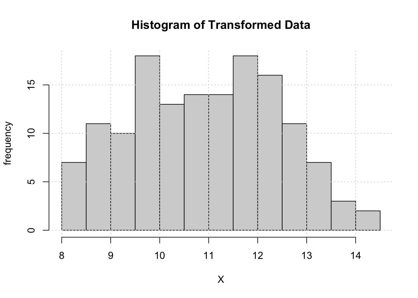
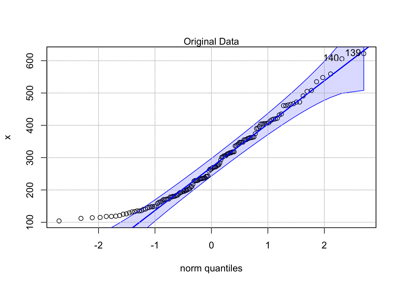
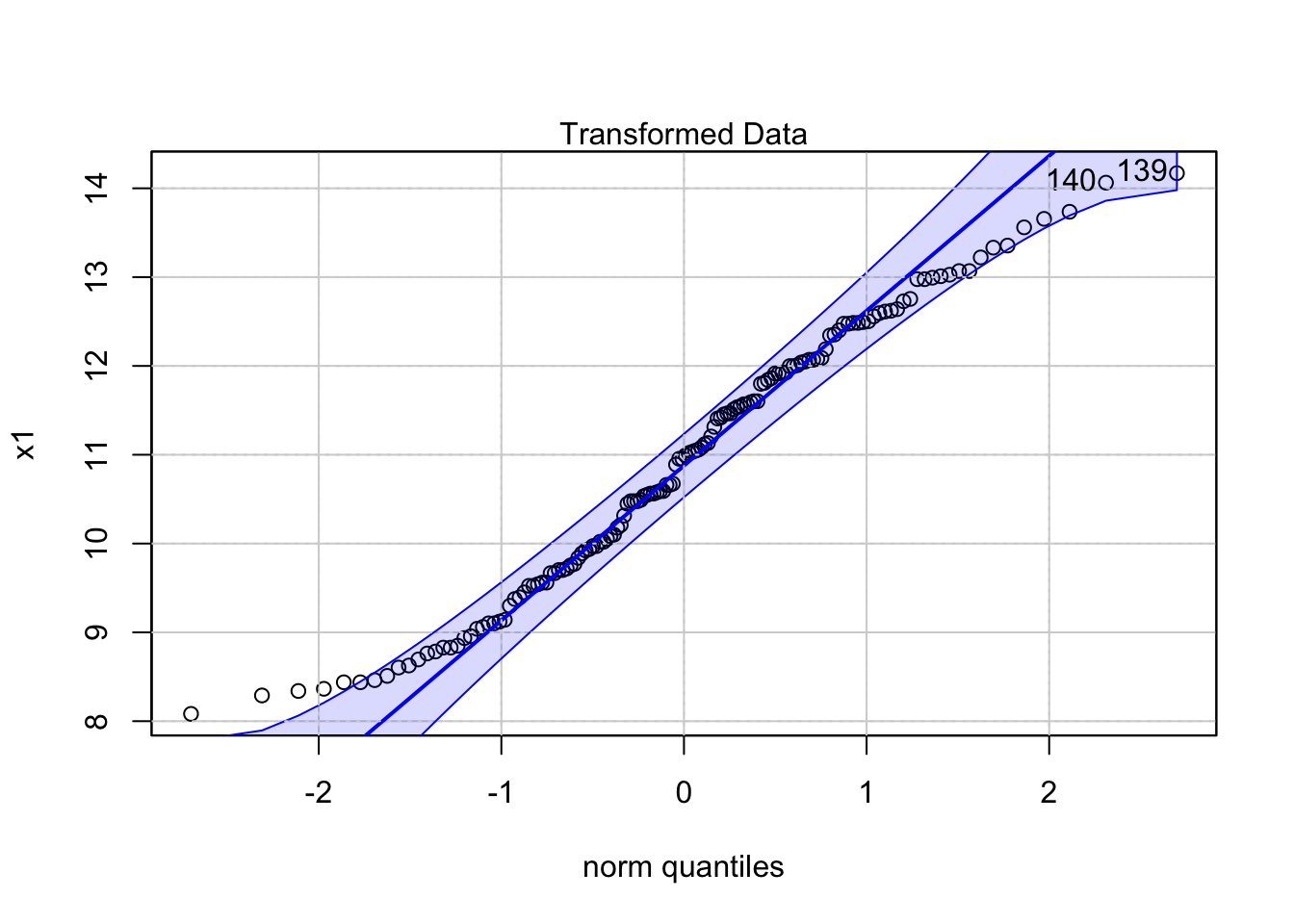
Consider the Airline time series which clearly exhibits a typical form of heteroskedasticity that can be removed through a Box-Cox transformation. The Box-Cox Normality Plot is shown in the following analysis and suggests that \(\lambda \simeq 0.22\) should be appropriate to induce normality2:

Interactive Shiny app (click to load).
Open in new tab

The output of the ML estimation shows that \(\lambda\) is (approximately) 0.148 with a 95% confidence interval of [-0.2374, 0.5335] which implies that \(\lambda\) is significantly different from 1 (\(p \simeq 1.59e-05\)) but not significantly different from 0 (\(p \simeq 0.45\)).

From the information shown above it is clear that the Box-Cox transform is able to induce approximate normality in the time series.

150.2.4 Example: Unemployment

Based on the SMP we identify the value for \(\lambda\) of the Box-Cox transformation.

Interactive Shiny app (click to load).
Open in new tab

The SMP shows that there is a significant relationship between the standard deviation and the mean of each year. The slope (\(\beta\)) of the regression line is significantly different from zero (\(p \simeq 0.0038\)), i.e. the Null Hypothesis H\(_0: \beta = 0\) is rejected. Hence it is necessary to apply a transformation which induces stationarity of the Variance. The quasi-optimal \(\lambda\) value is computed in the second regression model and is (approximately) equal to 0.47, which could be rounded to 0.5 (this corresponds to \(\sqrt{Y_t}\)). It is possible to apply this rounding because the Standard Deviation of \(\beta\) in the second model is (approximately) 0.115 which implies that \(\beta_0 = 0.5\) is contained in the 2-\(\sigma\) confidence interval around lambda: \(0.5 \in [0.467 - 2 \times 0.115, 0.467 + 2 \times 0.115]\), i.e. \(\lambda\) is not significantly different from 0.5.

We conclude that the Unemployment time series can be transformed in order to induce stationarity of the variance (\(\lambda = 0.5\)).

150.2.5 Example: Births

Based on the SMP we identify the value for \(\lambda\) of the Box-Cox transformation.

Interactive Shiny app (click to load).
Open in new tab

The SMP shows that there is no relationship between the standard deviation and the mean of subsequent years. Therefore, there is no need to apply the Box–Cox transformation (\(\lambda = 1\)).

150.2.6 Example: Soldiers

Based on the SMP we identify the value for \(\lambda\) of the Box-Cox transformation.

Interactive Shiny app (click to load).
Open in new tab

The SMP shows that there is no relationship between the standard deviation and the mean of sequential years. Therefore, there seems to be no need to apply the Box–Cox transformation (\(\lambda = 1\)).

Unfortunately, the SMP analysis for this time series might be somewhat misleading because the relationship between \(\sigma_i\) and \(\mu_i\) (for \(i = 1, 2, …,k\)) is probably not a linear one. The analysis clearly shows that the last year of the time series is drastically different from the previous years. Both \(\sigma_k\) and \(\mu_k\) are very small compared to the other years (the decision to withdraw troops from Iraq clearly resulted in fewer casualties). This can also be observed in the scatter plots of the analysis: the last year is shown in the bottom left area of the graph. If we would eliminate the last year from the computation, we would probably see a completely different regression line (one with a slightly negative slope).

We conclude that the SMP analysis is not always suited as a tool to find (quasi-)optimal values for \(\lambda\). The Simple Linear Regression Model can be (very) sensitive to outliers which may lead to wrong conclusions. We should always keep in mind that statistical methods make assumptions (which are not always satisfied).

150.2.7 Example: Traffic

Based on the SMP (with seasonality set to 7), we identify the value for \(\lambda\) of the Box-Cox transformation.

The SMP shows that there is a relationship between the standard deviation and the mean of sequential years. The slope (\(\beta\)) of the regression line is significantly different from zero (\(p \simeq 2e-16\)). The quasi-optimal \(\lambda\) value in the second regression equals -0.28 which cannot be rounded to 0 because the standard deviation is 0.08. In other words, the Traffic time series can be transformed in order to induce stationarity of the variance.

150.2.8 Example: Pageviews

To compute the SMP for the Pageviews time series we have to use a seasonality parameter of 7 instead of 12.

The SMP indicates a strong relationship between the standard deviation and the mean of sequential years. The slope (\(\beta\)) of the regression line is significantly different from zero (\(p < 2e-16\)). The quasi-optimal \(\lambda\) value can also be computed in a second regression (0.11) which must not be rounded to 0 because the standard deviation is only 0.036. In other words, the Pageviews time series should be transformed with \(\lambda = 0.11\) (i.e. \(Y_t^{0.11}\)) in order to induce stationarity.

150.3 Why do we need stationarity?

The most fundamental justification for time series analysis (as described in this chapter) is due to Wold’s decomposition theorem (Wold 1938). In practical terms, it states that a stationary time series can be decomposed into two parts: (1) a predictable component that is fully determined by past information, and (2) an innovation component driven by current and past shocks. The innovation component is generally represented as a one-sided moving-average expansion (not necessarily a finite-order MA model).

What does this all mean? In simple words, once stationarity has been induced, AR/MA/ARMA models provide useful finite approximations to the underlying dynamics. There is no general theorem guaranteeing that every arbitrary time series can be transformed into a stationary one. In applied work, however - especially for many economic time series - approximate stationarity can often be induced through transformations and differencing, but this should always be verified with diagnostics.

Box, George E. P., and David R. Cox. 1964. “An Analysis of Transformations.” Journal of the Royal Statistical Society. Series B (Methodological) 26 (2): 211–52. https://doi.org/10.1111/j.2517-6161.1964.tb00553.x.
Wold, Herman. 1938. A Study in the Analysis of Stationary Time Series. Uppsala: Almqvist & Wiksell.

  1. Actually, the time series could have multiple levels of seasonality (weekly, monthly, and annually). In this case, however, we limit ourselves to the investigation of weekly seasonality only.↩︎

  2. It is often the case that transforming data towards normality also helps to induce stationarity of the variance. Strictly speaking, however, normality and stationarity (of the variance) are not the same.↩︎

149  Theoretical Concepts
151  Identifying ARMA parameters

© 2026 Patrick Wessa. Provided as-is, without warranty.

Feedback: e-mail | Anonymous contributions: click to copy (Sats) | click to copy (XMR)

Cookie Preferences