• Descriptive
    • Moments
    • Concentration
    • Central Tendency
    • Variability
    • Stem-and-Leaf Plot
    • Histogram & Frequency Table
    • Data Quality Forensics
    • Conditional EDA
    • Quantiles
    • Kernel Density Estimation
    • Normal QQ Plot
    • Bootstrap Plot

    • Multivariate Descriptive Statistics
  • Distributions
    • Binomial Probabilities
    • Geometric Probabilities
    • Negative Binomial Probabilities
    • Hypergeometric Probabilities
    • Multinomial Probabilities
    • Dirichlet
    • Poisson Probabilities

    • Exponential
    • Gamma
    • Erlang
    • Weibull
    • Rayleigh
    • Maxwell-Boltzmann
    • Lognormal
    • Pareto
    • Inverse Gamma
    • Inverse Chi-Square

    • Beta
    • Power
    • Beta Prime (Inv. Beta)
    • Triangular

    • Normal (area)
    • Logistic
    • Laplace
    • Cauchy (standard)
    • Cauchy (location-scale)
    • Gumbel
    • Fréchet
    • Generalized Extreme Value

    • Normal RNG
    • ML Fitting
    • Tukey Lambda PPCC
    • Box-Cox Normality Plot
    • Noncentral t
    • Noncentral F
    • Sample Correlation r

    • Empirical Tests
  • Hypotheses
    • Theoretical Aspects of Hypothesis Testing
    • Bayesian Inference
    • Minimum Sample Size

    • Empirical Tests
    • Multivariate (pair-wise) Testing
  • Models
    • Manual Model Building
    • Guided Model Building
  • Time Series
    • Time Series Plot
    • Decomposition
    • Exponential Smoothing

    • Blocked Bootstrap Plot
    • Mean Plot
    • (P)ACF
    • VRM
    • Standard Deviation-Mean Plot
    • Spectral Analysis
    • ARIMA

    • Cross Correlation Function
    • Granger Causality
  1. Box-Jenkins Analysis
  2. 151  Identifying ARMA parameters
  • Preface
  • Getting Started
    • 1  Introduction
    • 2  Why Do We Need Innovative Technology?
    • 3  Basic Definitions
    • 4  The Big Picture: Why We Analyze Data
  • Introduction to Probability
    • 5  Definitions of Probability
    • 6  Jeffreys’ axiom system
    • 7  Bayes’ Theorem
    • 8  Sensitivity and Specificity
    • 9  Naive Bayes Classifier
    • 10  Law of Large Numbers

    • 11  Problems
  • Probability Distributions
    • 12  Bernoulli Distribution
    • 13  Binomial Distribution
    • 14  Geometric Distribution
    • 15  Negative Binomial Distribution
    • 16  Hypergeometric Distribution
    • 17  Multinomial Distribution
    • 18  Poisson Distribution

    • 19  Uniform Distribution (Rectangular Distribution)
    • 20  Normal Distribution (Gaussian Distribution)
    • 21  Gaussian Naive Bayes Classifier
    • 22  Chi Distribution
    • 23  Chi-squared Distribution (1 parameter)
    • 24  Chi-squared Distribution (2 parameters)
    • 25  Student t-Distribution
    • 26  Fisher F-Distribution
    • 27  Exponential Distribution
    • 28  Lognormal Distribution
    • 29  Gamma Distribution
    • 30  Beta Distribution
    • 31  Weibull Distribution
    • 32  Pareto Distribution
    • 33  Inverse Gamma Distribution
    • 34  Rayleigh Distribution
    • 35  Erlang Distribution
    • 36  Logistic Distribution
    • 37  Laplace Distribution
    • 38  Gumbel Distribution
    • 39  Cauchy Distribution
    • 40  Triangular Distribution
    • 41  Power Distribution
    • 42  Beta Prime Distribution
    • 43  Sample Correlation Distribution
    • 44  Dirichlet Distribution
    • 45  Generalized Extreme Value (GEV) Distribution
    • 46  Frechet Distribution
    • 47  Noncentral t Distribution
    • 48  Noncentral F Distribution
    • 49  Inverse Chi-Squared Distribution
    • 50  Maxwell-Boltzmann Distribution
    • 51  Distribution Relationship Map

    • 52  Problems
  • Descriptive Statistics & Exploratory Data Analysis
    • 53  Types of Data
    • 54  Datasheets

    • 55  Frequency Plot (Bar Plot)
    • 56  Frequency Table
    • 57  Contingency Table
    • 58  Binomial Classification Metrics
    • 59  Confusion Matrix
    • 60  ROC Analysis

    • 61  Stem-and-Leaf Plot
    • 62  Histogram
    • 63  Data Quality Forensics
    • 64  Quantiles
    • 65  Central Tendency
    • 66  Variability
    • 67  Skewness & Kurtosis
    • 68  Concentration
    • 69  Notched Boxplot
    • 70  Scatterplot
    • 71  Pearson Correlation
    • 72  Rank Correlation
    • 73  Partial Pearson Correlation
    • 74  Simple Linear Regression
    • 75  Moments
    • 76  Quantile-Quantile Plot (QQ Plot)
    • 77  Normal Probability Plot
    • 78  Probability Plot Correlation Coefficient Plot (PPCC Plot)
    • 79  Box-Cox Normality Plot
    • 80  Kernel Density Estimation
    • 81  Bivariate Kernel Density Plot
    • 82  Conditional EDA: Panel Diagnostics
    • 83  Bootstrap Plot (Central Tendency)
    • 84  Survey Scores Rank Order Comparison
    • 85  Cronbach Alpha

    • 86  Equi-distant Time Series
    • 87  Time Series Plot (Run Sequence Plot)
    • 88  Mean Plot
    • 89  Blocked Bootstrap Plot (Central Tendency)
    • 90  Standard Deviation-Mean Plot
    • 91  Variance Reduction Matrix
    • 92  (Partial) Autocorrelation Function
    • 93  Periodogram & Cumulative Periodogram

    • 94  Problems
  • Hypothesis Testing
    • 95  Normal Distributions revisited
    • 96  The Population
    • 97  The Sample
    • 98  The One-Sided Hypothesis Test
    • 99  The Two-Sided Hypothesis Test
    • 100  When to use a one-sided or two-sided test?
    • 101  What if \(\sigma\) is unknown?
    • 102  The Central Limit Theorem (revisited)
    • 103  Statistical Test of the Population Mean with known Variance
    • 104  Statistical Test of the Population Mean with unknown Variance
    • 105  Statistical Test of the Variance
    • 106  Statistical Test of the Population Proportion
    • 107  Statistical Test of the Standard Deviation \(\sigma\)
    • 108  Statistical Test of the difference between Means -- Independent/Unpaired Samples
    • 109  Statistical Test of the difference between Means -- Dependent/Paired Samples
    • 110  Statistical Test of the difference between Variances -- Independent/Unpaired Samples

    • 111  Hypothesis Testing for Research Purposes
    • 112  Decision Thresholds, Alpha, and Confidence Levels
    • 113  Bayesian Inference for Decision-Making
    • 114  One Sample t-Test
    • 115  Skewness & Kurtosis Tests
    • 116  Paired Two Sample t-Test
    • 117  Wilcoxon Signed-Rank Test
    • 118  Unpaired Two Sample t-Test
    • 119  Unpaired Two Sample Welch Test
    • 120  Two One-Sided Tests (TOST) for Equivalence
    • 121  Mann-Whitney U test (Wilcoxon Rank-Sum Test)
    • 122  Bayesian Two Sample Test
    • 123  Median Test based on Notched Boxplots
    • 124  Chi-Squared Tests for Count Data
    • 125  Kolmogorov-Smirnov Test
    • 126  One Way Analysis of Variance (1-way ANOVA)
    • 127  Kruskal-Wallis Test
    • 128  Two Way Analysis of Variance (2-way ANOVA)
    • 129  Repeated Measures ANOVA
    • 130  Friedman Test
    • 131  Testing Correlations
    • 132  A Note on Causality

    • 133  Problems
  • Regression Models
    • 134  Simple Linear Regression Model (SLRM)
    • 135  Multiple Linear Regression Model (MLRM)
    • 136  Logistic Regression
    • 137  Generalized Linear Models
    • 138  Multinomial and Ordinal Logistic Regression
    • 139  Cox Proportional Hazards Regression
    • 140  Conditional Inference Trees
    • 141  Leaf Diagnostics for Conditional Inference Trees
    • 142  Conditional Random Forests
    • 143  Hypothesis Testing with Linear Regression Models (from a Practical Point of View)

    • 144  Problems
  • Introduction to Time Series Analysis
    • 145  Case: the Market of Health and Personal Care Products
    • 146  Decomposition of Time Series
    • 147  Ad hoc Forecasting of Time Series
  • Box-Jenkins Analysis
    • 148  Introduction to Box-Jenkins Analysis
    • 149  Theoretical Concepts
    • 150  Stationarity
    • 151  Identifying ARMA parameters
    • 152  Estimating ARMA Parameters and Residual Diagnostics
    • 153  Forecasting with ARIMA models
    • 154  Intervention Analysis
    • 155  Cross-Correlation Function
    • 156  Transfer Function Noise Models
    • 157  General-to-Specific Modeling
  • Model Building Strategies
    • 158  Introduction to Model Building Strategies
    • 159  Manual Model Building
    • 160  Model Validation
    • 161  Regularization Methods
    • 162  Hyperparameter Optimization Strategies
    • 163  Guided Model Building in Practice
    • 164  Diagnostics, Revision, and Guided Forecasting
    • 165  Leakage, Target Encoding, and Robust Regression
  • References
  • Appendices
    • Appendices
    • A  Method Selection Guide
    • B  Presentations and Teaching Materials
    • C  R Language Concepts for Statistical Computing
    • D  Matrix Algebra
    • E  Standard Normal Table (Gaussian Table)
    • F  Critical values of Student’s \(t\) distribution with \(\nu\) degrees of freedom
    • G  Upper-tail critical values of the \(\chi^2\)-distribution with \(\nu\) degrees of freedom
    • H  Lower-tail critical values of the \(\chi^2\)-distribution with \(\nu\) degrees of freedom

Table of contents

  • 151.1 AR(1) Model
  • 151.2 AR(2) Model
  • 151.3 MA(1) Model
  • 151.4 MA(2) Model
  • 151.5 ARMA(1,1) Model
  • 151.6 ARMA Identification Summary
  • 151.7 Practical Identification Workflow
  • 151.8 Identifying ARMA Parameters in Practice
  1. Box-Jenkins Analysis
  2. 151  Identifying ARMA parameters

151  Identifying ARMA parameters

Any stationary time series can be modelled by AR and MA models as is shown in Wold’s decomposition theorem (Wold 1938). The definitions and properties of (some of) these models are described in the following sections.

151.1 AR(1) Model

The AR(1) process is defined as

\[ \begin{aligned} (1-\phi_1 B) W_t &= e_t \\ W_t - \phi_1 W_{t-1} &= e_t \\ W_t &= \phi_1 W_{t-1} + e_t \end{aligned} \]

where \(W_t\) is a stationary time series, \(e_t\) is a white noise error term, and \(F_t\) is called the forecast or prediction. Now we derive the theoretical pattern of the ACF of an AR(1) process for identification purposes.

First, we note that the above expression may be rewritten as follows

\[ \begin{aligned} (1 - \phi_1 B) W_t &= e_t \\ W_t &= (1 - \phi_1 B)^{-1} e_t \\ W_t &= e_t + \phi_1 e_{t-1} + \phi_1^2 e_{t-2} + \phi_1^3 e_{t-3} + \cdots \end{aligned} \]

We multiply the AR(1) process by \(W_{t-k}\) in expectations form

\[ \begin{aligned} W_t W_{t-k} - \phi_1 W_{t-1} W_{t-k} &= e_t W_{t-k} \\ \text{E}(W_t W_{t-k}) - \phi_1 \text{E}(W_{t-1} W_{t-k}) &= \text{E}(e_t W_{t-k}) \\ \gamma_k - \phi_1 \gamma_{k-1} &= \text{E}(e_t W_{t-k}) \end{aligned} \]

For \(k=0\), the right hand side may be rewritten as

\[ \begin{aligned} \text{E}(e_t W_t) &= \text{E} \left[ e_t ( e_t + \phi_1 e_{t-1} + \phi_1^2 e_{t-2} + \cdots ) \right] \\ \text{E}(e_t W_t) &= \text{E}(e_t^2) = \sigma_{e_t}^2 \end{aligned} \]

and for \(k>0\), the right hand side is

\[ \begin{aligned} \text{E}(e_t W_{t-k}) &= \text{E} \left[ e_t ( e_{t-k} + \phi_1 e_{t-k-1} + \phi_1^2 e_{t-k-2} + \cdots ) \right] \\ \text{E}(e_t W_{t-k}) &= 0 \end{aligned} \]

Hence, the left hand side becomes

\[ \gamma_k - \phi_1 \gamma_{k-1} = \begin{cases} \gamma_0 - \phi_1 \gamma_1 = \sigma_{e_t}^2 \text{ for } k = 0 \\ 0 \text{ for } k > 0 \end{cases} \]

Based on the previous expressions, we can investigate the characteristics of the ACF and PACF:

\[ \begin{aligned} \gamma_0 - \phi_1 \gamma_1 &= \sigma_{e_t}^2 \\ \gamma_0 - \phi_1^2 \gamma_0 &= \sigma_{e_t}^2 \\ \gamma_0 &= \frac{\sigma_{e_t}^2}{1 - \phi_1^2} \end{aligned} \]

and

\[ \begin{aligned} \gamma_k - \phi_1 \gamma_{k-1} &= 0 \\ \gamma_k &= \phi_1 \gamma_{k-1} \\ \frac{\gamma_k}{\gamma_0} &= \phi_1 \frac{\gamma_{k-1}}{\gamma_0} \end{aligned} \]

such that \(\rho_k = \phi_1 \rho_{k-1} = \phi_1^2 \rho_{k-2} = \phi_1^3 \rho_{k-3} = \cdots\). We conclude that \(\rho_k = \phi_1^k \rho_0 = \phi_1^k\).

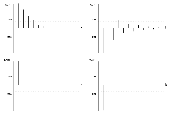
Figure 151.1: Theoretical ACF/PACF of AR(1) process

Figure 151.1 shows two theoretical patterns that occur in the ACF and PACF when the stationary time series \(W_t\) follows an AR(1) process. Note that the first ACF and PACF coefficients are always equal.

Generally speaking, a linear filter process is stationary if the inverse-filter expansion converges. For AR(1), stationarity requires \(|\phi_1|<1\). Equivalently, the root of \((1-\phi_1 B)=0\) is \(B=1/\phi_1\), which must lie outside the unit circle (absolute value greater than 1).

\[ \psi(B) = (1 - \phi_1 B)^{-1} = \sum_{j=0}^{\infty} \phi_1^j B^j \]

For a general AR(p) model the solutions of

\[ \phi(B) = \prod_{i=1}^{p} (1 - \xi_i B) \]

for which

\[ \forall i \in \{1,2,\ldots,p\}: \left|\xi_i\right| < 1 \]

must be satisfied in order to obtain stationarity.

Equivalent statement (often used in textbooks): if roots are written in the polynomial variable \(z\) for \(\\phi(z)=0\), those roots must lie outside the unit circle. Both formulations describe the same stationarity condition.

151.2 AR(2) Model

The AR(2) process is defined as

\[ \begin{align*}(1-\phi_1 B - \phi_2 B^2) W_t &= e_t \\W_t - \phi_1 W_{t-1} - \phi_2 W_{t-2} &= e_t \\W_t - e_t &= \phi_1 W_{t-1} + \phi_2 W_{t-2}\\F_t &= \phi_1 W_{t-1} + \phi_2 W_{t-2}\end{align*} \]

where \(W_t\) is a stationary time series, \(e_t\) is a white noise error term, and \(F_t\) is the forecasting function.

The process can be written in the form

\[ \begin{align*}(1-\phi_1 B - \phi_2 B^2) W_t &= e_t \\W_t &= (1 + \psi_1 B + \psi_2 B^2 + \psi_3 B^3 + …) e_t \\W_t &= \Psi(B) e_t\end{align*} \]

and therefore

\[ \begin{align*}(1 - \phi_1 B - \phi_2 B^2)^{-1} = \Psi(B) &= (1 + \psi_1 B + \psi_2 B^2 + \psi_3 B^3 + …) \\(1 - \phi_1 B - \phi_2 B^2)(1 + \psi_1 B + \psi_2 B^2 + \psi_3 B^3 + …) &= 1\end{align*} \]

For this to be valid, it follows that

\[ \psi_1 - \phi_1 = 0 \Leftrightarrow \psi_1 = \phi_1 \]

and that

\[ \psi_2 - \phi_1 \psi_1 - \phi_2 = 0 \Leftrightarrow \psi_2 = \phi_1^2 + \phi_2 \]

and that

\[ \psi_3 - \phi_1 \psi_2 - \phi_2 \psi_1 = 0 \Leftrightarrow \psi_3 = \phi_1^3 + 2 \phi_1 \phi_2 \]

and finally that

\[ \forall i \ge 3: \psi_i = \phi_1 \psi_{i-1} + \phi_2 \psi_{i-2} \]

The model is stationary if the \(\psi_i\) weights converge. This is the case when some conditions on \(\phi_1\) and \(\phi_2\) are imposed. These conditions can be found on using the solutions of the polynomial of the AR(2) model. The so-called characteristic equation is used to find these solutions

\[ (1 - \phi_1 B - \phi_2 B^2) = (1 - \xi_1 B)(1 - \xi_2 B) = 0 \]

The solutions of \(\xi_1\) and \(\xi_2\) are

\[ \xi_1, \xi_2 = \frac{\phi_1 \pm \sqrt{\phi_1^2 + 4 \phi_2}}{2} \]

which can be either real or complex. Note that the roots are complex if \(\phi_1^2 + 4 \phi_2 < 0\). When these solutions (in absolute values) are smaller than 1, the AR(2) model is stationary.

It can be shown that these conditions are satisfied if \(\phi_1\) and \(\phi_2\) lie inside of the Stralkowski triangular region which is restricted by

\[ \begin{cases} \phi_2 + \phi_1 < 1 \\ \phi_2 - \phi_1 < 1 \\ -1 < \phi_2 < 1 \\\end{cases} \]

The theoretical ACF and PACF are illustrated below.

Figure 151.2: Theoretical ACF/PACF of AR(2) process with real roots
Figure 151.3: Theoretical ACF/PACF of AR(2) process with complex roots

151.3 MA(1) Model

The MA(1) process is defined as

\[ \begin{align*}W_t &= (1 - \theta_1 B) e_t \\W_t &= e_t - \theta_1 e_{t-1}\end{align*} \]

Note

R’s arima() function uses the MA sign convention \((1 + \\theta_1 B)\), which is the opposite sign of the convention used in this chapter. Therefore, ma = c(-0.8) in R corresponds to \(\\theta_1 = 0.8\) here.

where \(W_t\) is a stationary time series and \(e_t\) is a white noise error term. The current observation depends on the current and previous error term. We now derive the theoretical ACF of the MA(1) process.

We compute the autocovariance at lag \(k\) by multiplying \(W_t\) by \(W_{t-k}\) in expectations form

\[ \begin{align*}\gamma_k &= \text{E}(W_t W_{t-k}) \\&= \text{E}\left[(e_t - \theta_1 e_{t-1})(e_{t-k} - \theta_1 e_{t-k-1})\right]\end{align*} \]

For \(k=0\)

\[ \gamma_0 = \text{E}(e_t^2) + \theta_1^2 \text{E}(e_{t-1}^2) = (1 + \theta_1^2) \sigma_{e_t}^2 \]

For \(k=1\)

\[ \gamma_1 = \text{E}\left[(e_t - \theta_1 e_{t-1})(e_{t-1} - \theta_1 e_{t-2})\right] = -\theta_1 \sigma_{e_t}^2 \]

For \(k > 1\), all expectations vanish because the error terms are uncorrelated: \(\gamma_k = 0\).

Therefore the ACF is

\[ \rho_k = \frac{\gamma_k}{\gamma_0} = \begin{cases} \dfrac{-\theta_1}{1 + \theta_1^2} & \text{for } k = 1 \\ 0 & \text{for } k > 1 \end{cases} \]

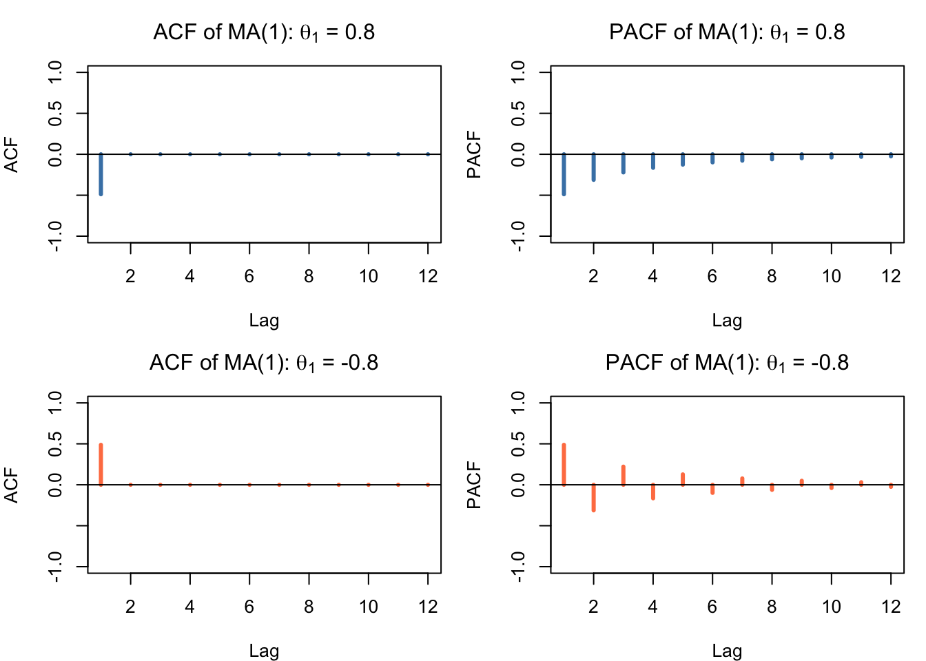
The ACF of an MA(1) process cuts off after lag 1, while the PACF shows an exponential decay (tailing off). This pattern is the mirror image of the AR(1) process where the ACF decays and the PACF cuts off.

The MA(1) model is invertible if the root of \((1 - \theta_1 B) = 0\) is larger than 1 in absolute value, which requires \(|\theta_1| < 1\). Invertibility ensures that the MA representation can be rewritten as an infinite AR process and guarantees uniqueness of the model.

par(mfrow = c(2, 2), mar = c(4, 4, 3, 1))
# MA(1) with positive theta
acf_vals <- ARMAacf(ma = c(-0.8), lag.max = 12)
pacf_vals <- ARMAacf(ma = c(-0.8), lag.max = 12, pacf = TRUE)
plot(1:12, acf_vals[-1], type = "h", lwd = 3, col = "steelblue",
     xlab = "Lag", ylab = "ACF", main = expression(paste("ACF of MA(1): ", theta[1], " = 0.8")),
     ylim = c(-1, 1))
abline(h = 0)
plot(1:12, pacf_vals, type = "h", lwd = 3, col = "steelblue",
     xlab = "Lag", ylab = "PACF", main = expression(paste("PACF of MA(1): ", theta[1], " = 0.8")),
     ylim = c(-1, 1))
abline(h = 0)
# MA(1) with negative theta
acf_vals2 <- ARMAacf(ma = c(0.8), lag.max = 12)
pacf_vals2 <- ARMAacf(ma = c(0.8), lag.max = 12, pacf = TRUE)
plot(1:12, acf_vals2[-1], type = "h", lwd = 3, col = "coral",
     xlab = "Lag", ylab = "ACF", main = expression(paste("ACF of MA(1): ", theta[1], " = -0.8")),
     ylim = c(-1, 1))
abline(h = 0)
plot(1:12, pacf_vals2, type = "h", lwd = 3, col = "coral",
     xlab = "Lag", ylab = "PACF", main = expression(paste("PACF of MA(1): ", theta[1], " = -0.8")),
     ylim = c(-1, 1))
abline(h = 0)
par(mfrow = c(1, 1))
Figure 151.4: Theoretical ACF/PACF of MA(1) process

151.4 MA(2) Model

The MA(2) process is defined as

\[ \begin{align*}W_t &= (1 - \theta_1 B - \theta_2 B^2) e_t \\W_t &= e_t - \theta_1 e_{t-1} - \theta_2 e_{t-2}\end{align*} \]

Following the same derivation as for the MA(1) model, the autocovariances are

\[ \begin{align*}\gamma_0 &= (1 + \theta_1^2 + \theta_2^2) \sigma_{e_t}^2 \\\gamma_1 &= (-\theta_1 + \theta_1 \theta_2) \sigma_{e_t}^2 \\\gamma_2 &= -\theta_2 \sigma_{e_t}^2 \\\gamma_k &= 0 \quad \text{for } k > 2\end{align*} \]

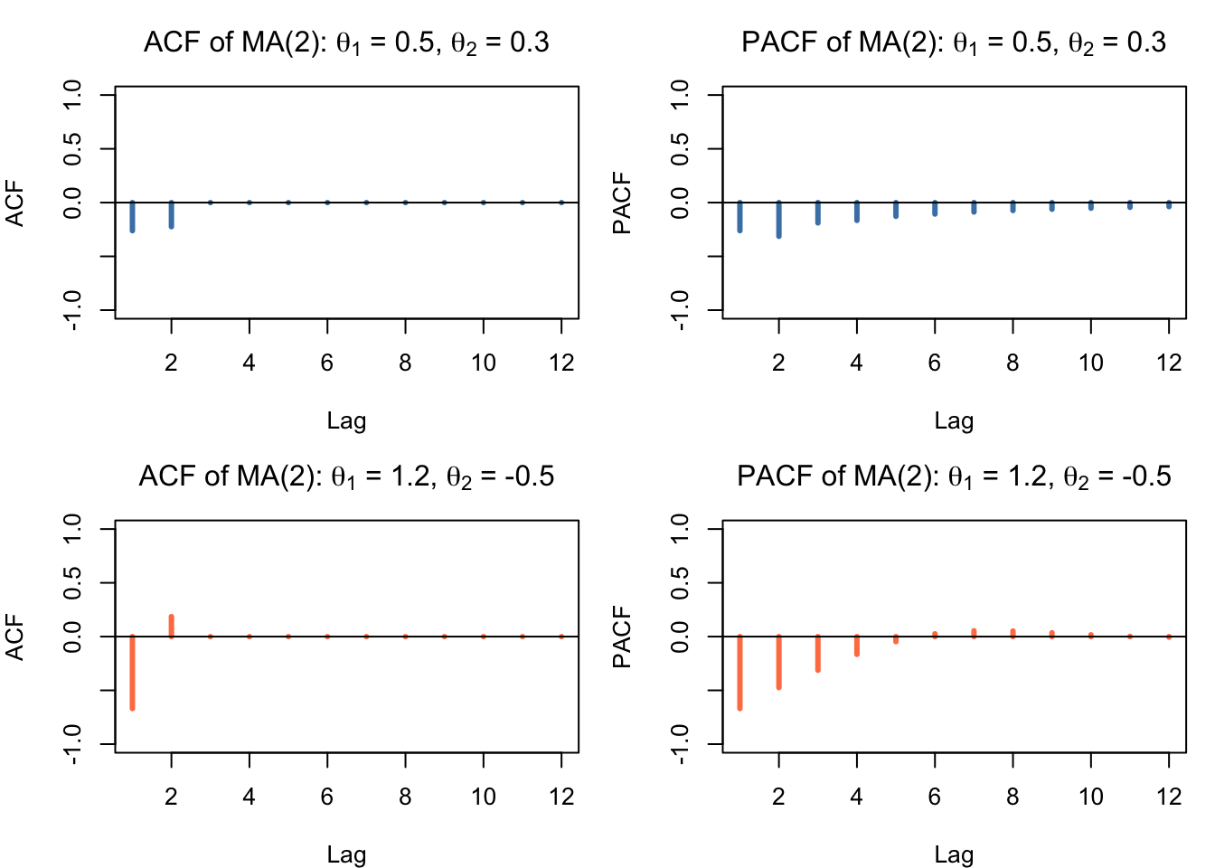
The ACF of an MA(2) process therefore cuts off after lag 2, while the PACF shows a decay pattern. The invertibility conditions require that the roots of the characteristic equation \((1 - \theta_1 B - \theta_2 B^2) = 0\) lie outside the unit circle, analogously to the stationarity conditions for the AR(2) model.

par(mfrow = c(2, 2), mar = c(4, 4, 3, 1))
acf_vals <- ARMAacf(ma = c(-0.5, -0.3), lag.max = 12)
pacf_vals <- ARMAacf(ma = c(-0.5, -0.3), lag.max = 12, pacf = TRUE)
plot(1:12, acf_vals[-1], type = "h", lwd = 3, col = "steelblue",
     xlab = "Lag", ylab = "ACF",
     main = expression(paste("ACF of MA(2): ", theta[1], " = 0.5, ", theta[2], " = 0.3")),
     ylim = c(-1, 1))
abline(h = 0)
plot(1:12, pacf_vals, type = "h", lwd = 3, col = "steelblue",
     xlab = "Lag", ylab = "PACF",
     main = expression(paste("PACF of MA(2): ", theta[1], " = 0.5, ", theta[2], " = 0.3")),
     ylim = c(-1, 1))
abline(h = 0)
acf_vals2 <- ARMAacf(ma = c(-1.2, 0.5), lag.max = 12)
pacf_vals2 <- ARMAacf(ma = c(-1.2, 0.5), lag.max = 12, pacf = TRUE)
plot(1:12, acf_vals2[-1], type = "h", lwd = 3, col = "coral",
     xlab = "Lag", ylab = "ACF",
     main = expression(paste("ACF of MA(2): ", theta[1], " = 1.2, ", theta[2], " = -0.5")),
     ylim = c(-1, 1))
abline(h = 0)
plot(1:12, pacf_vals2, type = "h", lwd = 3, col = "coral",
     xlab = "Lag", ylab = "PACF",
     main = expression(paste("PACF of MA(2): ", theta[1], " = 1.2, ", theta[2], " = -0.5")),
     ylim = c(-1, 1))
abline(h = 0)
par(mfrow = c(1, 1))
Figure 151.5: Theoretical ACF/PACF of MA(2) process

151.5 ARMA(1,1) Model

The ARMA(1,1) process combines both an AR(1) and MA(1) component

\[ \begin{align*}(1 - \phi_1 B) W_t &= (1 - \theta_1 B) e_t \\W_t - \phi_1 W_{t-1} &= e_t - \theta_1 e_{t-1}\end{align*} \]

The theoretical ACF of the ARMA(1,1) model has a starting value

\[ \rho_1 = \frac{(1 - \phi_1 \theta_1)(\phi_1 - \theta_1)}{1 + \theta_1^2 - 2 \phi_1 \theta_1} \]

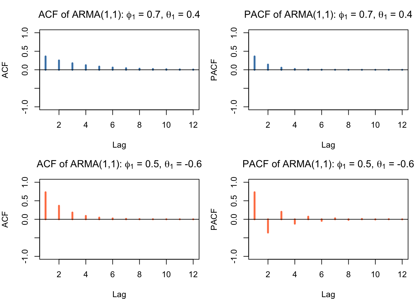
followed by exponential decay: \(\rho_k = \phi_1 \rho_{k-1}\) for \(k > 1\). The PACF also shows a decay pattern. Since both the ACF and PACF decay (neither cuts off cleanly), it is difficult in practice to identify an ARMA model from the ACF/PACF alone. This is precisely why the backward selection approach (Chapter 152) is so useful: rather than trying to identify exact values of \(p\) and \(q\) from theoretical patterns, we start with maximum values and let the estimation procedure eliminate non-significant parameters.

par(mfrow = c(2, 2), mar = c(4, 4, 3, 1))
acf_vals <- ARMAacf(ar = c(0.7), ma = c(-0.4), lag.max = 12)
pacf_vals <- ARMAacf(ar = c(0.7), ma = c(-0.4), lag.max = 12, pacf = TRUE)
plot(1:12, acf_vals[-1], type = "h", lwd = 3, col = "steelblue",
     xlab = "Lag", ylab = "ACF",
     main = expression(paste("ACF of ARMA(1,1): ", phi[1], " = 0.7, ", theta[1], " = 0.4")),
     ylim = c(-1, 1))
abline(h = 0)
plot(1:12, pacf_vals, type = "h", lwd = 3, col = "steelblue",
     xlab = "Lag", ylab = "PACF",
     main = expression(paste("PACF of ARMA(1,1): ", phi[1], " = 0.7, ", theta[1], " = 0.4")),
     ylim = c(-1, 1))
abline(h = 0)
acf_vals2 <- ARMAacf(ar = c(0.5), ma = c(0.6), lag.max = 12)
pacf_vals2 <- ARMAacf(ar = c(0.5), ma = c(0.6), lag.max = 12, pacf = TRUE)
plot(1:12, acf_vals2[-1], type = "h", lwd = 3, col = "coral",
     xlab = "Lag", ylab = "ACF",
     main = expression(paste("ACF of ARMA(1,1): ", phi[1], " = 0.5, ", theta[1], " = -0.6")),
     ylim = c(-1, 1))
abline(h = 0)
plot(1:12, pacf_vals2, type = "h", lwd = 3, col = "coral",
     xlab = "Lag", ylab = "PACF",
     main = expression(paste("PACF of ARMA(1,1): ", phi[1], " = 0.5, ", theta[1], " = -0.6")),
     ylim = c(-1, 1))
abline(h = 0)
par(mfrow = c(1, 1))
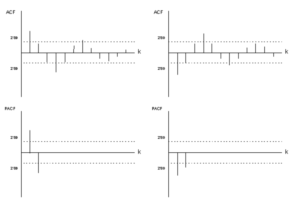
Figure 151.6: Theoretical ACF/PACF of ARMA(1,1) process

151.6 ARMA Identification Summary

The table below summarises the theoretical ACF and PACF patterns for the most common models. These patterns form the basis of the Box-Jenkins identification step.

Table 151.1: ACF/PACF identification patterns
Model ACF pattern PACF pattern
AR(1) Exponential decay Cuts off after lag 1
AR(2) Exponential or sinusoidal decay Cuts off after lag 2
AR(p) Decays (exponential and/or sinusoidal) Cuts off after lag p
MA(1) Cuts off after lag 1 Exponential decay
MA(2) Cuts off after lag 2 Exponential or sinusoidal decay
MA(q) Cuts off after lag q Decays (exponential and/or sinusoidal)
ARMA(p,q) Tails off (no clean cutoff) Tails off (no clean cutoff)

In practice, the sample ACF and PACF are noisy estimates of the theoretical patterns, making it hard to distinguish between “cutting off” and “decaying” especially for mixed ARMA models. This is why the ARIMA Backward Selection approach described in the next chapters is recommended as the primary identification strategy.

151.7 Practical Identification Workflow

In real datasets, a practical workflow is usually more reliable than pattern matching alone:

  1. Transform and difference first (\(\\lambda\), \(d\), \(D\)) so the working series is approximately stationary.
  2. Inspect ACF/PACF of the stationary series and propose small candidate sets for \((p,q,P,Q)\).
  3. Fit a deliberately general candidate (e.g., modest maxima for \(p,q,P,Q\)) and simplify.
  4. Compare candidates using information criteria (AIC/BIC; Akaike (1974); Schwarz (1978)) and residual diagnostics (ACF/PACF, Ljung-Box (Ljung and Box 1978), normality checks).
  5. Keep the most parsimonious model that passes diagnostics and still forecasts well out of sample.

This chapter focuses on Step 2 (theoretical identification patterns). The implementation of Steps 3–5 is provided in Chapter 152.

151.8 Identifying ARMA Parameters in Practice

The complete ARIMA(p,d,q)(P,D,Q)-lambda model is defined by the following equation:

\[ (1-\phi_1 B^1 -\phi_2 B^2 - ... - \phi_p B^p) (1-\Phi_1 B_s^1 - \Phi_2 B_s^2 - ... - \Phi_P B_s^P) \nabla^d \nabla_s^D \lambda(Y_t) \]

\[ = (1 - \theta_1 B^1 - \theta_2 B^2 - ... - \theta_q B^q) (1 - \Theta_1 B_s^1 - \Theta_2 B_s^2- ... - \Theta_Q B_s^Q) e_t \]

Before we can estimate the AR and MA parameters we need to identify the appropriate values for \(\lambda\), d, D, p, q, P, and Q. We already know how to determine \(\lambda\), d, and D. The other parameters may be identified through careful examination of the ACF and Partial ACF (PACF) about the stationary time series (for instance, the theoretical ACF and PACF patterns that correspond to the AR(1) process).

It requires a lot of experience to identify the values for p, q, P, and Q based on the theoretical patterns of AR and MA models. Therefore we introduce an easier method (ARIMA Backward selection) which is based on a trial-and-error strategy that simplifies a general model (see next section).

Akaike, Hirotugu. 1974. “A New Look at the Statistical Model Identification.” IEEE Transactions on Automatic Control 19 (6): 716–23. https://doi.org/10.1109/TAC.1974.1100705.
Ljung, Greta M., and George E. P. Box. 1978. “On a Measure of Lack of Fit in Time Series Models.” Biometrika 65 (2): 297–303. https://doi.org/10.1093/biomet/65.2.297.
Schwarz, Gideon. 1978. “Estimating the Dimension of a Model.” The Annals of Statistics 6 (2): 461–64. https://doi.org/10.1214/aos/1176344136.
Wold, Herman. 1938. A Study in the Analysis of Stationary Time Series. Uppsala: Almqvist & Wiksell.
150  Stationarity
152  Estimating ARMA Parameters and Residual Diagnostics

© 2026 Patrick Wessa. Provided as-is, without warranty.

Feedback: e-mail | Anonymous contributions: click to copy (Sats) | click to copy (XMR)

Cookie Preferences