The Chi-Squared Tests for Count Data which fall under the category of Pearson Chi-Squared Tests (Pearson 1900) can be subdivided in two types: a goodness-of-fit test and an independence test. The first type is based on a one dimensional test statistic and is typically used to test whether or not the observed frequencies differ from a theoretical distribution (e.g. a normality test). The second type is computed for two dimensional contingency tables and tests whether or not the variable represented in the rows are independent from the variable shown in the columns of the contingency table.
For continuous data, an alternative goodness-of-fit test is the Kolmogorov-Smirnov test (Chapter 125), which does not require binning the data into categories and preserves all information in the sample. When parameters are estimated from the same sample, use a Lilliefors-corrected KS test (nortest::lillie.test) or the Anderson-Darling test, because standard KS critical values are invalid in that case.
where \(O_i\) denotes the number of observations in category \(i\), \(E_i\) is the expected/theoretical frequency of type \(i\), and \(k\) is the number of categories. The test statistic of this type follows a Chi-Squared Distribution with degrees of freedom equal to \(k - p - 1\) where \(p\) is the number of parameters that is used to define the theoretical distribution (e.g. for the Normal Distribution \(p = 2\)).
The independence test statistic for a two dimension contingency table is defined as
where \(r\) is the number of rows, \(c\) is the number of columns, \(O_{ij}\) is the observed frequency in the \(i\)-th row of column \(j\), and \(E_{ij}\) is the expected frequency in the \(i\)-th row of column \(j\) of the contingency table. The test statistic of this type follows a Chi-Squared Distribution with degrees of freedom equal to \((r-1)(c-1)\).
Note that the Pearson Chi-Squared value is closely related to the Pearson Phi Coefficient or Matthews Correlation (Section 71.7) which is typically used for the Confusion Matrix of Binomial Classification problems (Chapter 58). The relationship can be formulated as follows:
\[
\phi^2 = \frac{\chi^2}{n}
\]
where \(n\) is the total number of observations.
124.1.1 Hypotheses
The Null Hypothesis states that observed frequencies match expected frequencies under the model.
For a goodness-of-fit setting: H\(_0\): the specified distribution fits the data.
For an independence setting: H\(_0\): the variables are independent.
The Alternative Hypothesis states that the distribution does not fit (goodness-of-fit) or that variables are associated (independence).
124.1.2 Analysis based on p-values -- Software
The Chi-Squared Test R module can be found on the publicly available website:
The R Module is also available in RFC under the “Hypotheses / Empirical Tests” menu item.
124.1.3 Analysis based on p-values -- Data & Parameters
This R module contains the following fields:
Data X: a multivariate dataset containing quantitative data
Names of X columns: a space delimited list of names (one name for each column)
Factor 1: a positive integer value of the column in the multivariate dataset which corresponds to the first sample
Factor 2: a positive integer value of the column in the multivariate dataset which corresponds to the second sample
Type of test to use. This parameter can be set to the following values:
Pearson Chi-Squared
Monte Carlo (simulation-based) Pearson Chi-Squared (labeled “Exact Pearson Chi-Squared by Simulation” in the module)
McNemar Chi-Squared
Stuart-Maxwell Marginal Homogeneity
Bowker Symmetry (McNemar-Bowker)
Fisher Exact Test
124.1.4 Analysis based on p-values -- Output
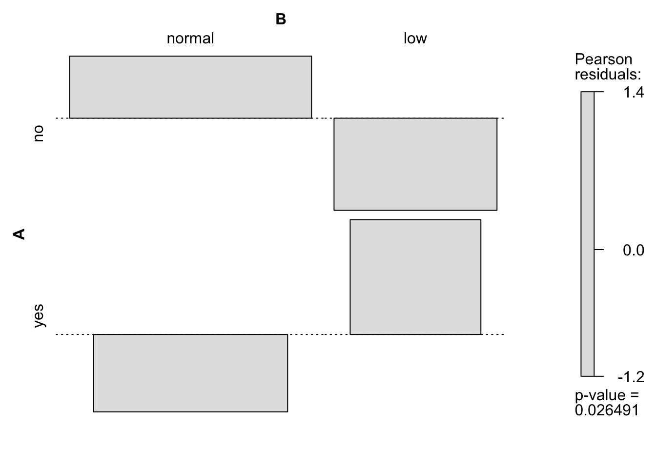
Consider the case where we wish to investigate the association between smoking and low birth weight of infants. Both variables are coded as binary numbers, i.e.:
low birth weight (\(< 2.5\) kg) corresponds to low = 1 (0 otherwise)
when the mother smokes cigarettes then smoke = 1 (0 otherwise)
The total number of observations and the expected cell frequencies are sufficiently large for the Pearson Chi-Squared Test to be used. The p-value is 3.958% which is (for most researchers) small enough to reject the Null Hypothesis. We conclude that smoking and low birth weight are associated.
For reporting, include an association effect size in addition to the p-value. For an \(r \times c\) table:
\[
V = \sqrt{\frac{\chi^2}{N\,\min(r-1, c-1)}}
\]
where \(V\) is Cramer’s \(V\)(Cramér 1946) (for \(2\times2\) tables, this reduces to \(\phi\)).
To compute the Chi-Squared Test on your local machine, the following script can be used in the R console:
library(MASS)library(vcd)x <- birthwtx$smoke <-factor(x$smoke, levels =c(0, 1), labels =c("no", "yes"))x$low <-factor(x$low, levels =c(0, 1), labels =c("normal", "low"))par3 ='Pearson Chi-Squared'#Type of test to usemain ='Association Plot'simulate.p.value=FALSEB =2000if (par3 %in%c('Monte Carlo (simulation-based) Pearson Chi-Squared','Exact Pearson Chi-Squared by Simulation')) simulate.p.value=TRUEcat("Actual frequencies\n")(table1 <-table(x$smoke, x$low))assoc(table1, shade =TRUE)
Actual frequencies

      normal low
  no      86  29
  yes     44  30

    Pearson's Chi-squared test with Yates' continuity correction

data:  table1
X-squared = 4.2359, df = 1, p-value = 0.03958


Expected frequencies

        normal      low
  no  79.10053 35.89947
  yes 50.89947 23.10053
124.2 Assumptions
The following assumptions are made:
The observations are obtained from a simple random sample.
The sample size must be sufficiently large.
For the Chi-Squared approximation to be reliable, no more than 20% of expected frequencies should be below 5 and none should be below 1; otherwise use a simulation-based Pearson test or Fisher’s Exact Test.
The observations are independent of each other. This also implies that the samples must be unpaired.
The main advantage of the Chi-Squared Tests is that it can be used with qualitative (i.e categorical) data. If one employs these tests with quantitative data, one must define categories first (which implies that information is lost).
124.3 Alternatives
If expected cell counts are too small, use Fisher’s Exact Test or the simulation-based Pearson test (both discussed below). For paired binary data, use McNemar’s Test. For paired square tables with more than two categories, use Stuart-Maxwell (marginal homogeneity) and/or Bowker (symmetry), depending on the hypothesis of interest.
If originally quantitative data were categorized, consider using methods on the original scale (e.g. correlation or regression) to avoid information loss.
124.4 Monte Carlo (Simulation-Based) Pearson Chi-Squared Test
124.4.1 Hypotheses
The hypotheses are identical to those of the Pearson Chi-Squared Test (Section 124.1).
124.4.2 Analysis based on p-values
Consider the survey results from many years ago. We wish to test whether there is a difference between female and male students when it comes to their favorite choice of Internet browser. In the R module shown below, select the AMS dataset in the Input tab, click on Chi-squared Test, select Browser as X variable, select gender as Y variable, and specify that you want the Monte Carlo (simulation-based) Pearson method (labeled “Exact Pearson Chi-Squared by Simulation” in the app) in the “Type of test to use” box.
The expected cell frequencies in the output Table are too low for the Pearson Chi-Squared Test to be used1. Therefore, it is necessary to use a Monte Carlo simulation method to obtain a reliable approximate p-value.
Using Monte Carlo simulation (\(B = 2000\) replicates), the p-value is rather small (approximately 3.298%) – therefore we reject the Null Hypothesis and conclude that the choice of browser is different for males and females. Results vary slightly across runs due to Monte Carlo simulation error. This contrast also shows how anti-conservative the Chi-squared approximation can become when expected cell counts are too low: if you select the ordinary Pearson Chi-squared method, the p-value drops to 0.1777%, implying that we could have come to an opposite conclusion if the chosen type I error would be 3% instead of 5%.
To compute the Chi-Squared Test by Simulation on your local machine, the following parameter should be changed in the previous script:
par3 ='Monte Carlo (simulation-based) Pearson Chi-Squared'B =2000
124.5 Assumptions
The assumptions are the same as for the Pearson Chi-Squared Test except for the requirement that the expected cell frequencies are sufficiently large.
124.6 Alternatives
This is the same as for the Pearson Chi-Squared Test.
124.7 Fisher’s Exact Test
Fisher’s Exact Test (Fisher 1935) is used to test the association between two categorical variables in a contingency table when sample sizes are small or when expected cell counts fall below 5. Unlike the Pearson Chi-Squared test, which relies on a large-sample approximation, Fisher’s Exact Test computes the exact p-value using the hypergeometric distribution.
124.7.1 When to Use
Fisher’s Exact Test is preferred over the Pearson Chi-Squared Test when:
One or more expected cell frequencies are less than 5
You want an exact p-value rather than an asymptotic approximation
For large samples with adequate expected cell counts, the Pearson Chi-Squared Test and Fisher’s Exact Test give virtually identical results. However, Fisher’s Exact Test is always valid regardless of sample size, while the Pearson approximation may be unreliable for small samples.
124.7.2 Hypotheses
The hypotheses are the same as for the Pearson Chi-Squared independence test (Section 124.1):
\[
H_0: \text{The two variables are independent (no association)}
\]
\[
H_A: \text{The two variables are not independent (there is an association)}
\]
124.7.3 How It Works
For a 2×2 contingency table, given fixed row and column totals (marginals), the probability of observing any particular table configuration follows the hypergeometric distribution:
\[
P = \frac{\binom{R_1}{a} \binom{R_2}{c}}{\binom{N}{C_1}}
\]
where \(a\) is the observed count in the first cell, \(c = C_1-a\) is the observed count in the second row/first column cell, \(R_1\) and \(R_2\) are the row totals, \(C_1\) is the first column total, and \(N\) is the grand total.
The p-value is computed as the sum of probabilities of all table configurations that are as extreme as, or more extreme than, the observed table.
Contingency Table:
         Outcome
Treatment Improved Not improved
  Drug           3            1
  Placebo        1            5

Expected frequencies:
         Outcome
Treatment Improved Not improved
  Drug         1.6          2.4
  Placebo      2.4          3.6

Fisher's Exact Test:

    Fisher's Exact Test for Count Data

data:  treatment_table
p-value = 0.1905
alternative hypothesis: true odds ratio is not equal to 1
95 percent confidence interval:
   0.40161 930.24692
sample estimates:
odds ratio
  10.29391
Note that several expected cell frequencies are below 5, making the Pearson Chi-Squared approximation unreliable. Fisher’s Exact Test provides a valid p-value in this situation.
124.7.6 Assumptions
The observations are independent
The row and column totals (marginals) are fixed by the study design, or treated as fixed for the purpose of inference
The data are categorical (nominal or ordinal)
124.7.7 When to Prefer Over Pearson Chi-Squared
Table 124.1: Choosing between Pearson Chi-Squared and Fisher’s Exact Test
Situation
Recommended Test
All expected counts \(\geq\) 5
Pearson Chi-Squared (faster, same result)
Any expected count \(<\) 5
Fisher’s Exact Test
Large, sparse contingency table
Fisher’s Exact Test (or simulation-based Pearson)
124.8 Association vs. Marginal Homogeneity vs. Symmetry
For count data, three related but distinct null hypotheses are common:
\[
H_0^{\text{ind}}: X \perp Y \quad \text{(independence / association question)}
\]
\[
H_0^{\text{mh}}: \pi_{i+} = \pi_{+i}\ \forall i \quad \text{(marginal homogeneity in paired square tables)}
\]
\[
H_0^{\text{sym}}: \pi_{ij} = \pi_{ji}\ \forall i \neq j \quad \text{(symmetry in paired square tables)}
\]
In plain language:
Independence asks whether row and column variables are associated in an unpaired table.
Marginal homogeneity asks whether pre/post (or rater A/rater B) marginal distributions are equal in a paired square table.
Symmetry asks whether opposite transition cells are equal: \((i \rightarrow j)\) versus \((j \rightarrow i)\).
124.8.1 Choosing the test
Data structure
Main null hypothesis
Recommended test
2×2 unpaired
Independence
Pearson Chi-Squared / Fisher Exact
2×2 paired
Marginal homogeneity (equiv. symmetry for 2×2)
McNemar
\(k\times k\) paired (\(k>2\))
Marginal homogeneity
Stuart-Maxwell (optionally Bhapkar)
\(k\times k\) paired (\(k>2\))
Symmetry
Bowker (McNemar-Bowker)
Key nuance:
For 2×2 paired tables, McNemar, marginal homogeneity, and symmetry coincide.
For \(k>2\) paired tables, Bowker (symmetry) and Stuart-Maxwell/Bhapkar (marginal homogeneity) are different hypotheses and can lead to different conclusions.
WarningCommon Pitfalls
Using Pearson independence on paired data and calling it a paired alternative to McNemar.
Treating Bowker symmetry and Stuart-Maxwell marginal homogeneity as interchangeable for \(k>2\).
Ignoring small expected counts in unpaired 2×2 tables (use Fisher or simulation when needed).
Interpreting Yates-corrected and uncorrected Pearson outputs as “contradictory” instead of approximation choices.
Reporting only p-values without an effect-size scale (e.g., odds ratio, risk difference, Cramer’s \(V\)).
Interpreting non-rejection of \(H_0\) as proof that assumptions hold exactly.
124.9 Worked Examples
124.9.1 Example A (2×2, unpaired association): Smoking vs low birth weight
# Explicit 2x2 table (rows = smoking, cols = low birth weight)tabA <-matrix(c(30, 44,29, 86),nrow =2, byrow =TRUE,dimnames =list(Smoking =c("Yes", "No"),LowBirthWeight =c("Low", "Normal")))tabA# Pearson (with and without Yates correction)chisq.test(tabA, correct =TRUE)chisq.test(tabA, correct =FALSE)# Simulation-based Pearson p-valueset.seed(1)chisq.test(tabA, simulate.p.value =TRUE, B =1e5)# Fisher exact testfisher.test(tabA)# Effect size: odds ratio (with CI from Fisher) and risk differenceor_fit <-fisher.test(tabA, conf.level =0.95)risk_smoke <- tabA["Yes", "Low"] /sum(tabA["Yes", ])risk_no <- tabA["No", "Low"] /sum(tabA["No", ])rd <- risk_smoke - risk_nocat("\nOdds ratio estimate (smoking vs non-smoking, low birth weight):",unname(or_fit$estimate), "\n")cat("95% CI for odds ratio:",paste(round(or_fit$conf.int, 4), collapse =" to "), "\n")cat("Risk difference (P(low|smoke) - P(low|no smoke)):", round(rd, 4), "\n")
       LowBirthWeight
Smoking Low Normal
    Yes  30     44
    No   29     86

    Pearson's Chi-squared test with Yates' continuity correction

data:  tabA
X-squared = 4.2359, df = 1, p-value = 0.03958


    Pearson's Chi-squared test

data:  tabA
X-squared = 4.9237, df = 1, p-value = 0.02649


    Pearson's Chi-squared test with simulated p-value (based on 1e+05
    replicates)

data:  tabA
X-squared = 4.9237, df = NA, p-value = 0.03717


    Fisher's Exact Test for Count Data

data:  tabA
p-value = 0.03618
alternative hypothesis: true odds ratio is not equal to 1
95 percent confidence interval:
 1.028780 3.964904
sample estimates:
odds ratio
  2.014137


Odds ratio estimate (smoking vs non-smoking, low birth weight): 2.014137
95% CI for odds ratio: 1.0288 to 3.9649
Risk difference (P(low|smoke) - P(low|no smoke)): 0.1532
124.9.2 Example B (2×2, paired outcomes): same students in Maths vs Stats
tabB <-matrix(c(52, 8,18, 42),nrow =2, byrow =TRUE,dimnames =list(Maths =c("Pass", "Fail"),Stats =c("Pass", "Fail")))tabB# Correct paired test (McNemar)mcnemar.test(tabB, correct =TRUE)# Exact McNemar via Binomial on discordant pairsb <- tabB["Pass", "Fail"]c <- tabB["Fail", "Pass"]cat("\nDiscordant pairs: b =", b, ", c =", c, "\n")binom.test(x = b, n = b + c, p =0.5, alternative ="two.sided")# Independence test on the same table (different question)chisq.test(tabB, correct =FALSE)cat("\nNote: Pearson independence here tests association, not paired change asymmetry.\n")
      Stats
Maths  Pass Fail
  Pass   52    8
  Fail   18   42

    McNemar's Chi-squared test with continuity correction

data:  tabB
McNemar's chi-squared = 3.1154, df = 1, p-value = 0.07756


Discordant pairs: b = 8 , c = 18

    Exact binomial test

data:  b and b + c
number of successes = 8, number of trials = 26, p-value = 0.07552
alternative hypothesis: true probability of success is not equal to 0.5
95 percent confidence interval:
 0.1432600 0.5178964
sample estimates:
probability of success
             0.3076923


    Pearson's Chi-squared test

data:  tabB
X-squared = 39.634, df = 1, p-value = 3.063e-10


Note: Pearson independence here tests association, not paired change asymmetry.
124.9.3 Example C (\(k\times k\), paired): marginal homogeneity via Stuart-Maxwell
tabC <-matrix(c(150, 54, 21,27, 138, 42,12, 48, 108),nrow =3, byrow =TRUE,dimnames =list(Pre =c("Low", "Medium", "High"),Post =c("Low", "Medium", "High")))tabCstuart_maxwell_manual <-function(tab) {# Stuart-Maxwell statistic:# X^2 = d' V^{-1} d# d_i = row_i - col_i (for i = 1,...,k-1)# V_ii = row_i + col_i - 2*n_ii# V_ij = -(n_ij + n_ji), i != j tab <-as.matrix(tab)stopifnot(nrow(tab) ==ncol(tab), nrow(tab) >=2) k <-nrow(tab) r <-rowSums(tab) c <-colSums(tab) d <- r - c idx <-seq_len(k -1) V <-matrix(0, nrow = k -1, ncol = k -1)for(i inseq_len(k -1)) { ii <- idx[i] V[i, i] <- r[ii] + c[ii] -2* tab[ii, ii]for(j inseq_len(k -1)) {if(i == j) next jj <- idx[j] V[i, j] <-- (tab[ii, jj] + tab[jj, ii]) } } d_red <- d[idx] stat <-as.numeric(t(d_red) %*%solve(V) %*% d_red) df <- k -1 p <-pchisq(stat, df = df, lower.tail =FALSE)list(statistic = stat, df = df, p.value = p, margins =cbind(row = r, col = c, diff = d))}sm <-stuart_maxwell_manual(tabC)sm$marginscat(sprintf("\nStuart-Maxwell: X-squared = %.4f, df = %d, p-value = %.6g\n", sm$statistic, sm$df, sm$p.value))if(requireNamespace("DescTools", quietly =TRUE)) {cat("\nValidation (DescTools::StuartMaxwellTest):\n")print(DescTools::StuartMaxwellTest(tabC))}
        Post
Pre      Low Medium High
  Low    150     54   21
  Medium  27    138   42
  High    12     48  108
       row col diff
Low    225 189   36
Medium 207 240  -33
High   168 171   -3

Stuart-Maxwell: X-squared = 11.8539, df = 2, p-value = 0.00266665
124.9.4 Example D (\(k\times k\), paired): symmetry via Bowker (McNemar-Bowker)
        Post
Pre      Low Medium High
  Low     80     30    5
  Medium  10     70   22
  High    25      2   75
Stuart-Maxwell (marginal homogeneity): X-squared = 0.0000, df = 2, p-value = 1
Bowker (symmetry): X-squared = 40.0000, df = 3, p-value = 1.06551e-08

Interpretation: margins can be equal while symmetry fails.
In this example, row and column margins are equal (Stuart-Maxwell does not reject), but opposite off-diagonal transitions are not equal (Bowker rejects). This demonstrates explicitly that for \(k>2\), marginal homogeneity and symmetry are different hypotheses.
Cramér, Harald. 1946. Mathematical Methods of Statistics. Princeton Mathematical Series 9. Princeton: Princeton University Press.
Fisher, Ronald A. 1935. The Design of Experiments. Edinburgh: Oliver; Boyd.
Pearson, Karl. 1900. “On the Criterion That a Given System of Deviations from the Probable in the Case of a Correlated System of Variables Is Such That It Can Be Reasonably Supposed to Have Arisen from Random Sampling.”The London, Edinburgh, and Dublin Philosophical Magazine and Journal of Science 50 (302): 157–75. https://doi.org/10.1080/14786440009463897.
Note that there are three columns for gender because one respondent left the gender field blank.↩︎