Code
x <- seq(-5,17,length=1000)
hx <- dnorm(x, mean = 5, sd = 2)
plot(x, hx, type="l", xlab="X", ylab="f(X)", xlim=c(-5,17), main="Normal density", sub = "(location = 5 and scale = 2)")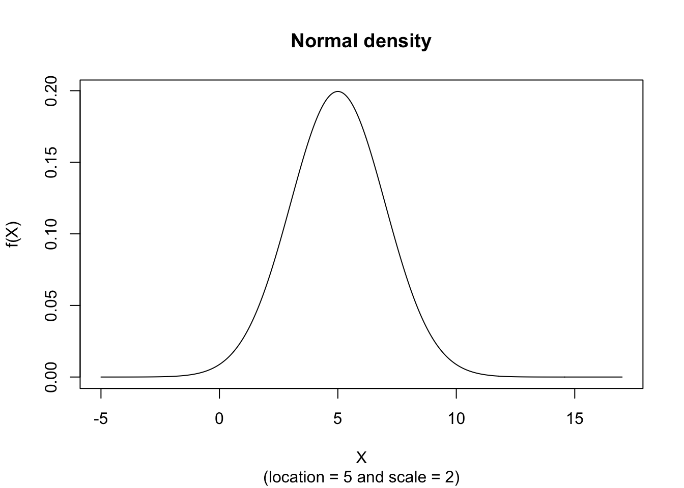
The random variate \(X\) defined for the range \(-\infty \leq X \leq +\infty\), is said to have a Normal Distribution (i.e. \(X \sim \text{N}\left( \mu, \sigma^2 \right)\)) with location parameter \(\mu\) and scale parameter \(\sigma\) where \(-\infty \leq \mu \leq +\infty\) and \(\sigma > 0\).
\[ \text{f}(X) = \frac{e^{-\frac{1}{2} \left( \frac{X - \mu}{\sigma} \right)^2} }{\sigma \sqrt{2 \pi}} \]
The figure below shows an example of the Normal Probability Density function with \(location = 5\) and \(scale = 2\).
x <- seq(-5,17,length=1000)
hx <- dnorm(x, mean = 5, sd = 2)
plot(x, hx, type="l", xlab="X", ylab="f(X)", xlim=c(-5,17), main="Normal density", sub = "(location = 5 and scale = 2)")\[ \text{F}(x) = \frac{1}{\sigma \sqrt{2 \pi}} \int_{-\infty}^{x} e^{- \frac{(t-\mu)^2}{2 \sigma^2}} \text{d}t \]
The figure below shows an example of the Normal Distribution with \(location = 5\) and \(scale = 2\).
x <- seq(-5,17,length=1000)
hx <- pnorm(x, mean = 5, sd = 2)
plot(x, hx, type="l", xlab="X", ylab="F(X)", xlim=c(-5,17), main="Normal distribution", sub = "(location = 5 and scale = 2)")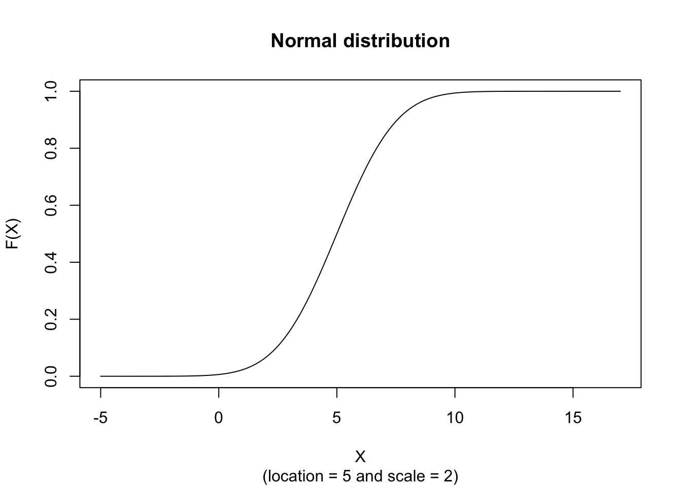
\[ M_X(t) = e^{\mu t + \frac{1}{2} \sigma^2 t^2 } \]
\[ \mu_1' = \mu \]
\[ \mu_2' = \mu^2 + \sigma^2 \]
\[ \mu_3' = \mu \left( \mu^2 + 3 \sigma^2 \right) \]
\[ \mu_4' = \mu^4 + 6 \mu^2 \sigma^2 + 3 \sigma^4 \]
\[ \mu_j = 0 \text{ for $j$ is odd} \]
\[ \mu_j = \frac{j!}{\left( \frac{j}{2} \right) ! \, 2^{\left( \frac{j}{2} \right)}} \sigma^j \text{ for $j$ even} \]
\[ \mu_2 = \sigma^2 \]
\[ \mu_3 = 0 \]
\[ \mu_4 = 3 \sigma^4 \]
\[ \text{E}(X) = \mu \]
\[ \text{V}(X) = \sigma^2 \]
\[ \text{Med}(X) = \mu \]
\[ \text{Mo}(X) = \mu \]
\[ g_1 = 0 \]
\[ g_2 = 3 \]
\[ VC = \frac{\sigma}{\mu} \]
\[ \hat{\mu}_{ML} = \bar{x} \text{ (maximum likelihood and unbiased)} \]
\[ \hat{\sigma}^2_{ML} = \frac{1}{n}\sum_{i=1}^{n} \left( x_i - \bar{x} \right)^2 \text{ (biased maximum likelihood)} \]
\[ \hat{\sigma}^2_{\text{unb}} = \frac{1}{n-1}\sum_{i=1}^{n} \left( x_i - \bar{x} \right)^2 = \frac{n}{n-1}\hat{\sigma}^2_{ML} \text{ (unbiased estimator)} \]
where
\[ \bar{x} = \frac{1}{n} \sum_{i=1}^{n} x_i \]
where \(s^2=\hat{\sigma}^2_{\text{unb}}\) denotes the usual sample variance.
The best fitting Normal Density function can be obtained by estimating \(\mu\) and \(\sigma\) according to the so-called Maximum Likelihood procedure which can be found on the public website:
The Maximum Likelihood Fitting for the Normal Distribution is also available in RFC under the menu “Distributions / ML Fitting”.
If you prefer to compute the Maximum Likelihood procedure on your local computer, there are two code snippets that can be pasted into the R console as an example. First we need to install the library “MASS” (you only need to do this once):
install.packages("MASS")Once the library has been installed, we can use the following code to perform Maximum Likelihood fitting:
library(MASS)
x <- runif(n = 1000) # draw Uniform random numbers
r <- fitdistr(x,'normal')
print(r)
mean sd
0.517353337 0.285413521
(0.009025568) (0.006382040)par1 = 8
par2 = 'Sturges'
ylab = 'density'
xlab = 'value of data series'
main = 'Histogram and Fitted Normal Density'
myhist<-hist(x, col=par1, breaks=par2, main=main, ylab=ylab, xlab=xlab, freq=F)
curve(1/(r$estimate[2]*sqrt(2*pi))*exp(-1/2*((x-r$estimate[1])/r$estimate[2])**2), min(x), max(x), add=T)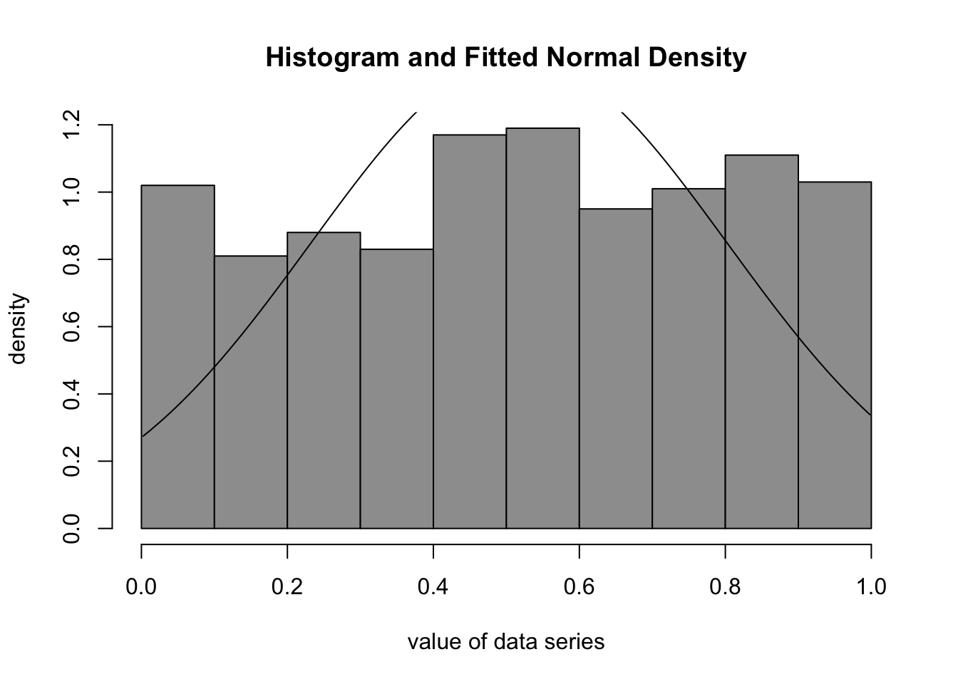
The par2 parameter defines the suggested number of bins of the Histogram (see Chapter 62). Mostly, however, we use the value ‘Sturges’ (default) to have the function compute the number of bins according to the Sturges algorithm (Sturges 1926).
The main functions in this example are hist (displays a histogram), curve (draws the curve of the Normal Density), and fitdistr (performs the actual Maximum Likelihood fitting).
We analyze the time series of monthly divorces (in thousands) and wish to find out whether it can be adequately described by the Normal Distribution. The Normal Density function seems to be a good fit for the Histogram of monthly divorces:
The visual fit suggests that a Normal model may be reasonable for the monthly divorces, with an approximate mean of 2.55 and standard deviation of 0.367 (the series is expressed in thousands of divorces). A formal goodness-of-fit assessment is still recommended; see Section 2, Section 124.1, and Chapter 125.
If U\((0,1)\) denotes a random variate with a Uniform Distribution (such as the pseudo random numbers generated by a digital computer) then the following approximation can be made arbitrarily accurate with increasing \(k\):
\[ \text{N}(0,1) \sim \frac{\sum_{i=1}^{k} \text{U}_i(0,1) - \frac{k}{2}}{\sqrt{\frac{k}{12}}} \]
For instance, if \(k=12\) then we can generate standard normally distributed random numbers
\[ \text{N}(0,1) \sim \sum_{i=1}^{12} \text{U}_i(0,1) - 6 \]
This is a classical pedagogical approximation. In practice, modern software (including rnorm) uses more accurate and efficient algorithms.
Based on random numbers for the Standard Normal Distribution, it is possible to obtain random numbers for any \(\mu \in \mathbb{R}\) and \(\sigma \in \mathbb{R}_0^+\) by using the following relationship
\[ \text{N}(\mu, \sigma^2) \sim \sigma \text{N}(0,1) + \mu \]
The Random Number Generator for the Normal Density function can be found on the public website:
The Random Number Generator for the Normal Distribution is also available in RFC under the menu “Distributions / Random Numbers - Normal” (this only applies when using the “default” profile).
If you prefer to generate Normal Random Numbers on your local computer, the following code snippet can be used in the R console1:
library(MASS)
library(msm)

par1 = 100
par2 = 0
par3 = 1
par4 = 2
par5 = 'N'
par6 = 'Sturges'
par7 = -Inf
par8 = Inf

ylab = 'density'
xlab = 'value of generated random numbers'
main = 'Histogram of Generated Random Numbers'
x <- rtnorm(par1, par2, par3, par7, par8)
if ((par7 == -Inf) & (par8 == Inf)) {r <- fitdistr(x,'normal')}

if (par5 == 'Y') {
  print(x)
}

print(r)
mean sd
-0.09163643 1.01272177
( 0.10127218) ( 0.07161024)The figure below shows that the Normal Density function fits the simulated data well:
myhist<-hist(x, col=par4, breaks=par6, main=main, ylab=ylab, xlab=xlab, freq=F)
curve(1/(r$estimate[2]*sqrt(2*pi))*exp(-1/2*((x-r$estimate[1])/r$estimate[2])^2), min(x), max(x), add=T)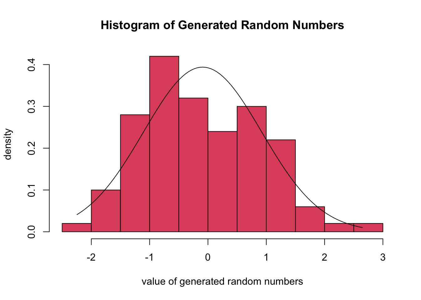
The script produces a Histogram and the associated Normal Density function (through ML Fitting) of the randomly generated numbers. The meaning and interpretation of histograms is discussed in detail in Chapter 62.
Note that it is also possible to use the rnorm function to simulate Normal Random Numbers without the need to use an external library:
rnorm(100, 5, 3) [1] 1.80146963 5.72827816 6.64020840 8.06626891 3.90505032 4.66242374
[7] 10.68673293 6.87140362 7.21619634 -0.45364789 3.08694423 3.04299449
[13] 9.28591171 1.46463016 6.43009863 3.84759329 7.51820999 2.98670249
[19] 7.99945949 9.31963394 0.76697681 6.42897400 2.96185209 3.86503586
[25] 3.96417560 6.87898579 9.40502125 6.82999246 3.24913022 7.97651724
[31] 12.12138487 -0.57738367 2.88003792 3.35775581 1.68154266 4.65089070
[37] 5.67606925 7.20485927 5.35622295 5.59702326 9.51918296 3.79305549
[43] -1.59563704 -1.03299289 3.09224787 5.03424843 6.60488757 5.44012700
[49] 5.78650990 7.06111925 4.02781026 8.12799522 8.53180293 4.73445934
[55] 8.53278646 0.14166071 7.12359374 -0.74107671 0.05044067 5.89235414
[61] 4.46457704 4.64367813 4.26147831 6.10202576 5.51251864 2.01261172
[67] 0.91416541 3.85836795 4.31122417 1.99095529 0.98057469 6.02385594
[73] -1.66843826 5.72516051 10.36533374 8.75029876 3.38458474 8.53401889
[79] 3.76968161 1.83985212 7.88771530 12.30605187 2.18277025 -0.25162244
[85] 2.73415245 3.85685737 5.64841719 10.83260860 3.91195816 3.76252340
[91] 5.94851330 6.92957409 3.15594003 1.37834661 7.04974441 1.29819657
[97] 4.20479365 3.27524250 9.29777534 -1.48975071Sometimes we prefer to use the rtnorm function (from the msm package) because this provides the option to use a truncation interval (i.e. a lower and upper bound for the random numbers that are generated). If par7 = -Inf (minus infinity) and par8 = Inf (infinity) then the rtnorm function produces similar results as the rnorm function (when the number of simulated values is sufficiently large).
We generate a series of 100 random numbers for the Normal Distribution with \(\mu = 5\) and \(\sigma = 2\). The Figure from the R Module shows the Histogram of the random numbers and the best fitting Normal Density curve.
The estimated parameters are obtained through ML Fitting and show the best fitting mean and standard deviation. It can be concluded that the empirical mean and standard deviation are close to the true values that are specified with the sliders. When the number of simulations increases, the empirical and true values will be closer together.
The Standard Normal Distribution is a Normal Distribution with zero mean (\(\mu = 0\)) and unit variance (\(\sigma^2 = \sigma = 1\)).
As \(\sigma \rightarrow 0\) then Normal Distribution becomes degenerate at \(\mu\).
The normally distributed variate \(X \sim \text{N}(\mu, \sigma^2)\) is symmetrical about \(\mu\) with points of inflection at \(X = \mu \pm \sigma\).
The sum of \(k\) independent variates which have a Normal Distribution N\(\left( \mu, \sigma^2 \right)\), is also Normally Distributed with mean \(k \mu\) and variance \(k \sigma^2\).
Let \(X_i\) (for \(i = 1, 2, …, k\)) be \(k\) normal variates with mean \(\mu_i\) and variance \(\sigma_i^2\) then \(\sum_{i=1}^{k} c_i X_i\) is also normally distributed with mean \(\mu = \sum_{i=1}^{k} c_i \mu_i\) and variance \(\sigma^2 = \sum_{i=1}^{k} c_i^2 \sigma_i^2\) where \(c_i\) (for \(i=1, 2, …, k\)) are weighting factors.
Suppose that the joint distribution of \(X_i\) (for \(i= 1, 2, …, k\)) is multivariate normal and let \(\mu_i = \text{E} \left( X_i \right)\) and \(c_{ij} = \text{Cov} \left(X_i, X_j\right)\) then it follows that for any \(a \in \mathbb{R}\) and \(b_i \in \mathbb{R}\) (for \(i=1, 2, …, k\)) the random variate \(Z = a + \sum_{i=1}^{k} b_i X_i\) has a Normal Distribution with expected value \(\mu = a + \sum_{i=1}^{k} b_i \mu_i\) and variance \(\sigma^2 = \sum_{i=1}^{k} \sum_{j=1}^{k} b_i b_j c_{ij}\).
This property also holds whether the variates \(X_i\) are independent or not. However, in case of independence, the variance becomes \(\sigma^2 = \sum_{i=1}^{k} b_i^2 V(X_i)\).
There are several random processes which can be assumed to have a Normal Distribution. This is of particular importance within the context of Hypothesis Testing which is extensively discussed in Hypothesis Testing. The Normal Distribution can also be used to extend the Multinomial Naive Bayes model from Chapter 9 so that continuous features can be used in addition to binary and count-based features.
Make sure that the MASS and msm packages have been installed with the install.packages function before running the script.↩︎