• Descriptive
    • Moments
    • Concentration
    • Central Tendency
    • Variability
    • Stem-and-Leaf Plot
    • Histogram & Frequency Table
    • Data Quality Forensics
    • Conditional EDA
    • Quantiles
    • Kernel Density Estimation
    • Normal QQ Plot
    • Bootstrap Plot

    • Multivariate Descriptive Statistics
  • Distributions
    • Binomial Probabilities
    • Geometric Probabilities
    • Negative Binomial Probabilities
    • Hypergeometric Probabilities
    • Multinomial Probabilities
    • Dirichlet
    • Poisson Probabilities

    • Exponential
    • Gamma
    • Erlang
    • Weibull
    • Rayleigh
    • Maxwell-Boltzmann
    • Lognormal
    • Pareto
    • Inverse Gamma
    • Inverse Chi-Square

    • Beta
    • Power
    • Beta Prime (Inv. Beta)
    • Triangular

    • Normal (area)
    • Logistic
    • Laplace
    • Cauchy (standard)
    • Cauchy (location-scale)
    • Gumbel
    • Fréchet
    • Generalized Extreme Value

    • Normal RNG
    • ML Fitting
    • Tukey Lambda PPCC
    • Box-Cox Normality Plot
    • Noncentral t
    • Noncentral F
    • Sample Correlation r

    • Empirical Tests
  • Hypotheses
    • Theoretical Aspects of Hypothesis Testing
    • Bayesian Inference
    • Minimum Sample Size

    • Empirical Tests
    • Multivariate (pair-wise) Testing
  • Models
    • Manual Model Building
    • Guided Model Building
  • Time Series
    • Time Series Plot
    • Decomposition
    • Exponential Smoothing

    • Blocked Bootstrap Plot
    • Mean Plot
    • (P)ACF
    • VRM
    • Standard Deviation-Mean Plot
    • Spectral Analysis
    • ARIMA

    • Cross Correlation Function
    • Granger Causality
  1. Box-Jenkins Analysis
  2. 153  Forecasting with ARIMA models
  • Preface
  • Getting Started
    • 1  Introduction
    • 2  Why Do We Need Innovative Technology?
    • 3  Basic Definitions
    • 4  The Big Picture: Why We Analyze Data
  • Introduction to Probability
    • 5  Definitions of Probability
    • 6  Jeffreys’ axiom system
    • 7  Bayes’ Theorem
    • 8  Sensitivity and Specificity
    • 9  Naive Bayes Classifier
    • 10  Law of Large Numbers

    • 11  Problems
  • Probability Distributions
    • 12  Bernoulli Distribution
    • 13  Binomial Distribution
    • 14  Geometric Distribution
    • 15  Negative Binomial Distribution
    • 16  Hypergeometric Distribution
    • 17  Multinomial Distribution
    • 18  Poisson Distribution

    • 19  Uniform Distribution (Rectangular Distribution)
    • 20  Normal Distribution (Gaussian Distribution)
    • 21  Gaussian Naive Bayes Classifier
    • 22  Chi Distribution
    • 23  Chi-squared Distribution (1 parameter)
    • 24  Chi-squared Distribution (2 parameters)
    • 25  Student t-Distribution
    • 26  Fisher F-Distribution
    • 27  Exponential Distribution
    • 28  Lognormal Distribution
    • 29  Gamma Distribution
    • 30  Beta Distribution
    • 31  Weibull Distribution
    • 32  Pareto Distribution
    • 33  Inverse Gamma Distribution
    • 34  Rayleigh Distribution
    • 35  Erlang Distribution
    • 36  Logistic Distribution
    • 37  Laplace Distribution
    • 38  Gumbel Distribution
    • 39  Cauchy Distribution
    • 40  Triangular Distribution
    • 41  Power Distribution
    • 42  Beta Prime Distribution
    • 43  Sample Correlation Distribution
    • 44  Dirichlet Distribution
    • 45  Generalized Extreme Value (GEV) Distribution
    • 46  Frechet Distribution
    • 47  Noncentral t Distribution
    • 48  Noncentral F Distribution
    • 49  Inverse Chi-Squared Distribution
    • 50  Maxwell-Boltzmann Distribution
    • 51  Distribution Relationship Map

    • 52  Problems
  • Descriptive Statistics & Exploratory Data Analysis
    • 53  Types of Data
    • 54  Datasheets

    • 55  Frequency Plot (Bar Plot)
    • 56  Frequency Table
    • 57  Contingency Table
    • 58  Binomial Classification Metrics
    • 59  Confusion Matrix
    • 60  ROC Analysis

    • 61  Stem-and-Leaf Plot
    • 62  Histogram
    • 63  Data Quality Forensics
    • 64  Quantiles
    • 65  Central Tendency
    • 66  Variability
    • 67  Skewness & Kurtosis
    • 68  Concentration
    • 69  Notched Boxplot
    • 70  Scatterplot
    • 71  Pearson Correlation
    • 72  Rank Correlation
    • 73  Partial Pearson Correlation
    • 74  Simple Linear Regression
    • 75  Moments
    • 76  Quantile-Quantile Plot (QQ Plot)
    • 77  Normal Probability Plot
    • 78  Probability Plot Correlation Coefficient Plot (PPCC Plot)
    • 79  Box-Cox Normality Plot
    • 80  Kernel Density Estimation
    • 81  Bivariate Kernel Density Plot
    • 82  Conditional EDA: Panel Diagnostics
    • 83  Bootstrap Plot (Central Tendency)
    • 84  Survey Scores Rank Order Comparison
    • 85  Cronbach Alpha

    • 86  Equi-distant Time Series
    • 87  Time Series Plot (Run Sequence Plot)
    • 88  Mean Plot
    • 89  Blocked Bootstrap Plot (Central Tendency)
    • 90  Standard Deviation-Mean Plot
    • 91  Variance Reduction Matrix
    • 92  (Partial) Autocorrelation Function
    • 93  Periodogram & Cumulative Periodogram

    • 94  Problems
  • Hypothesis Testing
    • 95  Normal Distributions revisited
    • 96  The Population
    • 97  The Sample
    • 98  The One-Sided Hypothesis Test
    • 99  The Two-Sided Hypothesis Test
    • 100  When to use a one-sided or two-sided test?
    • 101  What if \(\sigma\) is unknown?
    • 102  The Central Limit Theorem (revisited)
    • 103  Statistical Test of the Population Mean with known Variance
    • 104  Statistical Test of the Population Mean with unknown Variance
    • 105  Statistical Test of the Variance
    • 106  Statistical Test of the Population Proportion
    • 107  Statistical Test of the Standard Deviation \(\sigma\)
    • 108  Statistical Test of the difference between Means -- Independent/Unpaired Samples
    • 109  Statistical Test of the difference between Means -- Dependent/Paired Samples
    • 110  Statistical Test of the difference between Variances -- Independent/Unpaired Samples

    • 111  Hypothesis Testing for Research Purposes
    • 112  Decision Thresholds, Alpha, and Confidence Levels
    • 113  Bayesian Inference for Decision-Making
    • 114  One Sample t-Test
    • 115  Skewness & Kurtosis Tests
    • 116  Paired Two Sample t-Test
    • 117  Wilcoxon Signed-Rank Test
    • 118  Unpaired Two Sample t-Test
    • 119  Unpaired Two Sample Welch Test
    • 120  Two One-Sided Tests (TOST) for Equivalence
    • 121  Mann-Whitney U test (Wilcoxon Rank-Sum Test)
    • 122  Bayesian Two Sample Test
    • 123  Median Test based on Notched Boxplots
    • 124  Chi-Squared Tests for Count Data
    • 125  Kolmogorov-Smirnov Test
    • 126  One Way Analysis of Variance (1-way ANOVA)
    • 127  Kruskal-Wallis Test
    • 128  Two Way Analysis of Variance (2-way ANOVA)
    • 129  Repeated Measures ANOVA
    • 130  Friedman Test
    • 131  Testing Correlations
    • 132  A Note on Causality

    • 133  Problems
  • Regression Models
    • 134  Simple Linear Regression Model (SLRM)
    • 135  Multiple Linear Regression Model (MLRM)
    • 136  Logistic Regression
    • 137  Generalized Linear Models
    • 138  Multinomial and Ordinal Logistic Regression
    • 139  Cox Proportional Hazards Regression
    • 140  Conditional Inference Trees
    • 141  Leaf Diagnostics for Conditional Inference Trees
    • 142  Conditional Random Forests
    • 143  Hypothesis Testing with Linear Regression Models (from a Practical Point of View)

    • 144  Problems
  • Introduction to Time Series Analysis
    • 145  Case: the Market of Health and Personal Care Products
    • 146  Decomposition of Time Series
    • 147  Ad hoc Forecasting of Time Series
  • Box-Jenkins Analysis
    • 148  Introduction to Box-Jenkins Analysis
    • 149  Theoretical Concepts
    • 150  Stationarity
    • 151  Identifying ARMA parameters
    • 152  Estimating ARMA Parameters and Residual Diagnostics
    • 153  Forecasting with ARIMA models
    • 154  Intervention Analysis
    • 155  Cross-Correlation Function
    • 156  Transfer Function Noise Models
    • 157  General-to-Specific Modeling
  • Model Building Strategies
    • 158  Introduction to Model Building Strategies
    • 159  Manual Model Building
    • 160  Model Validation
    • 161  Regularization Methods
    • 162  Hyperparameter Optimization Strategies
    • 163  Guided Model Building in Practice
    • 164  Diagnostics, Revision, and Guided Forecasting
    • 165  Leakage, Target Encoding, and Robust Regression
  • References
  • Appendices
    • Appendices
    • A  Method Selection Guide
    • B  Presentations and Teaching Materials
    • C  R Language Concepts for Statistical Computing
    • D  Matrix Algebra
    • E  Standard Normal Table (Gaussian Table)
    • F  Critical values of Student’s \(t\) distribution with \(\nu\) degrees of freedom
    • G  Upper-tail critical values of the \(\chi^2\)-distribution with \(\nu\) degrees of freedom
    • H  Lower-tail critical values of the \(\chi^2\)-distribution with \(\nu\) degrees of freedom

Table of contents

  • 153.1 Example: Unemployment
    • 153.1.1 Generic Local Template (AirPassengers placeholder)
  • 153.2 Example: Births
  • 153.3 Example: Soldiers
  • 153.4 Example: Traffic
  • 153.5 Beyond Ceteris Paribus
  1. Box-Jenkins Analysis
  2. 153  Forecasting with ARIMA models

153  Forecasting with ARIMA models

In this section we use the estimated ARIMA models to generate ceteris paribus forecasts. Each forecast computation is obtained by:

  • cutting off the last s periods
  • generating an extrapolation forecast (without using the observations that were cut off)
  • comparing the extrapolation forecast against the actual values

Note that for each computation the actual/adequate values for \(\lambda\), d, D, p, q, P, and Q are used.

In this chapter:

  • short run refers to the first 1–12 forecast periods after the cut-off,
  • long run refers to horizons beyond 12 periods.

Forecast quality is summarised using standard error metrics:

  • MAPE / SMAPE for relative percentage errors,
  • MASE for scale-free comparison against a naive benchmark (Hyndman and Koehler 2006),
  • RMSE for squared-error sensitivity to large misses.

153.1 Example: Unemployment

Interactive Shiny app (click to load).
Open in new tab

The computation shown above (click on the Forecast tab first!) allows us to conclude that:

  • the expected forecast uncertainty is small on the short run (4%) and relatively high on the long run (28%)
  • the actual forecast error is much smaller than the expected error
  • the ceteris paribus conditions are satisfied during the last 12 months (there were no exceptional events)

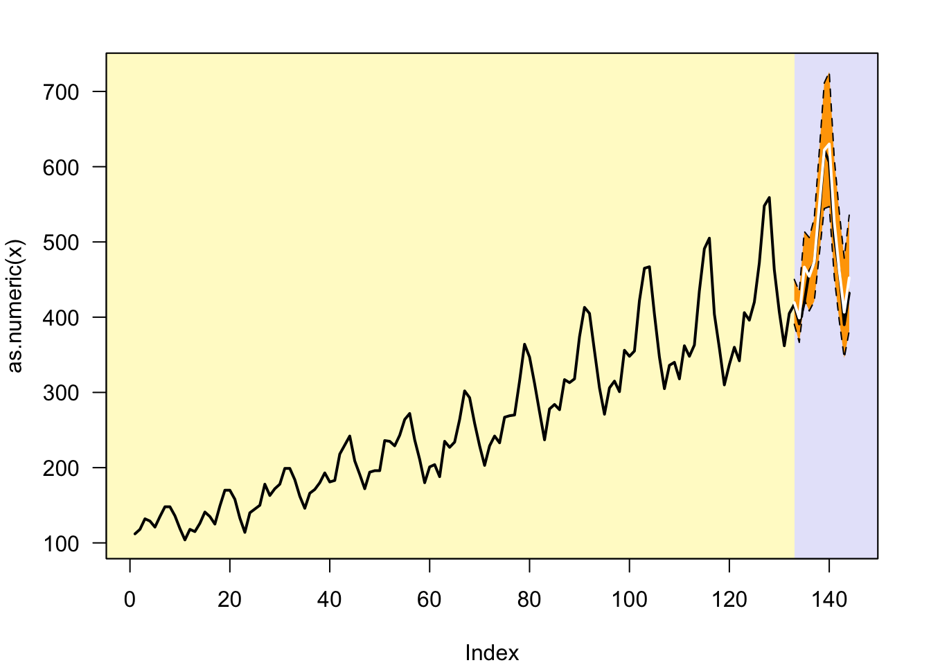
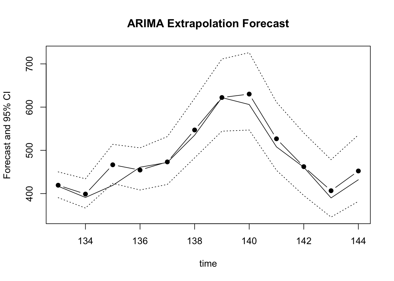
The extrapolation forecast clearly captures the seasonal pattern and the local trend, as can be observed in the figure near the bottom of the output. The figure also shows that the forecast track is closely aligned with the actual values from the cut-off period. In addition, the actual values are included in the 95% prediction intervals, indicating that the observed forecast errors are compatible with the model’s expected uncertainty for \(t = 361, 362, …, 372\).

153.1.1 Generic Local Template (AirPassengers placeholder)

If you prefer to compute ARIMA forecasting on your local machine, the following script is intentionally generic. It uses AirPassengers as a placeholder dataset.

To replicate this chapter’s Unemployment example, replace x <- AirPassengers with the Unemployment series and keep the same ARIMA settings.

library(lattice)
x <- AirPassengers  # placeholder dataset for the generic template
par1 = 12 #cut off periods
par2 = 0.0 #Box-Cox lambda transformation parameter
par3 = 1 #degree of non-seasonal differencing
par4 = 1 #degree of seasonal differencing
par5 = 12 #seasonal period
par6 = 0 #degree (p) of the non-seasonal AR(p) polynomial
par7 = 1 #degree (q) of the non-seasonal MA(q) polynomial
par8 = 0 #degree (P) of the seasonal AR(P) polynomial
par9 = 1 #degree (Q) of the seasonal MA(Q) polynomial
par10 = FALSE #Include mean?
if (par2 == 0) x <- log(x)
if (par2 != 0) x <- x^par2
lx <- length(x)
first <- lx - 2*par1
nx <- lx - par1
nx1 <- nx + 1
fx <- lx - nx
if (fx < 1) {
  fx <- par5*2
  nx1 <- lx + fx - 1
  first <- lx - 2*fx
}
first <- 1
if (fx < 3) fx <- round(lx/10,0)
arima.out <- arima(x[1:nx], order=c(par6,par3,par7), seasonal=list(order=c(par8,par4,par9), period=par5), include.mean=par10, method='ML')
forecast <- predict(arima.out,fx)
lb <- forecast$pred - 1.96 * forecast$se
ub <- forecast$pred + 1.96 * forecast$se
if (par2 == 0) {
  x <- exp(x)
  forecast$pred <- exp(forecast$pred)
  lb <- exp(lb)
  ub <- exp(ub)
}
if (par2 != 0) {
  x <- x^(1/par2)
  forecast$pred <- forecast$pred^(1/par2)
  lb <- lb^(1/par2)
  ub <- ub^(1/par2)
}
if (par2 < 0) {
  olb <- lb
  lb <- ub
  ub <- olb
}
actandfor <- c(x[1:nx], forecast$pred)
perc.se <- (ub-forecast$pred)/1.96/forecast$pred
opar <- par(mar=c(4,4,2,2),las=1)
ylim <- c( min(x[first:nx],lb), max(x[first:nx],ub))
plot(as.numeric(x),ylim=ylim,type='n',xlim=c(first,lx))
usr <- par('usr')
rect(usr[1],usr[3],nx+1,usr[4],border=NA,col='lemonchiffon')
rect(nx1,usr[3],usr[2],usr[4],border=NA,col='lavender')
abline(h= (-3:3)*2 , col ='gray', lty =3)
polygon( c(nx1:lx,lx:nx1), c(lb,rev(ub)), col = 'orange', lty=2,border=NA)
lines(nx1:lx, lb , lty=2)
lines(nx1:lx, ub , lty=2)
lines(as.numeric(x), lwd=2)
lines(nx1:lx, forecast$pred , lwd=2 , col ='white')
box()

par(opar)
prob.dec <- array(NA, dim=fx)
prob.sdec <- array(NA, dim=fx)
prob.ldec <- array(NA, dim=fx)
prob.pval <- array(NA, dim=fx)
perf.pe <- array(0, dim=fx)
perf.spe <- array(0, dim=fx)
perf.scalederr <- array(0, dim=fx)
perf.mase <- array(0, dim=fx)
perf.mase1 <- array(0, dim=fx)
perf.mape <- array(0, dim=fx)
perf.smape <- array(0, dim=fx)
perf.mape1 <- array(0, dim=fx)
perf.smape1 <- array(0,dim=fx)
perf.se <- array(0, dim=fx)
perf.mse <- array(0, dim=fx)
perf.mse1 <- array(0, dim=fx)
perf.rmse <- array(0, dim=fx)
perf.scaleddenom <- 0
for (i in 2:fx) {
  perf.scaleddenom = perf.scaleddenom + abs(x[nx+i] - x[nx+i-1])
}
perf.scaleddenom = perf.scaleddenom / (fx-1)
for (i in 1:fx) {
  locSD <- (ub[i] - forecast$pred[i]) / 1.96
  perf.scalederr[i] = (x[nx+i] - forecast$pred[i]) / perf.scaleddenom
  perf.pe[i] = (x[nx+i] - forecast$pred[i]) / x[nx+i]
  perf.spe[i] = 2*(x[nx+i] - forecast$pred[i]) / (x[nx+i] + forecast$pred[i])
  perf.se[i] = (x[nx+i] - forecast$pred[i])^2
  prob.dec[i] = pnorm((x[nx+i-1] - forecast$pred[i]) / locSD)
  prob.sdec[i] = pnorm((x[nx+i-par5] - forecast$pred[i]) / locSD)
  prob.ldec[i] = pnorm((x[nx] - forecast$pred[i]) / locSD)
  prob.pval[i] = pnorm(abs(x[nx+i] - forecast$pred[i]) / locSD)
}
perf.mape[1] = abs(perf.pe[1])
perf.smape[1] = abs(perf.spe[1])
perf.mape1[1] = perf.mape[1]
perf.smape1[1] = perf.smape[1]
perf.mse[1] = perf.se[1]
perf.mase[1] = abs(perf.scalederr[1])
perf.mase1[1] = perf.mase[1]
for (i in 2:fx) {
  perf.mape[i] = perf.mape[i-1] + abs(perf.pe[i])
  perf.mape1[i] = perf.mape[i] / i
  perf.smape[i] = perf.smape[i-1] + abs(perf.spe[i])
  perf.smape1[i] = perf.smape[i] / i
  perf.mse[i] = perf.mse[i-1] + perf.se[i]
  perf.mse1[i] = perf.mse[i] / i
  perf.mase[i] = perf.mase[i-1] + abs(perf.scalederr[i])
  perf.mase1[i] = perf.mase[i] / i
}
perf.rmse = sqrt(perf.mse1)
plot(forecast$pred, pch=19, type='b',main='ARIMA Extrapolation Forecast', ylab='Forecast and 95% CI', xlab='time',ylim=c(min(lb),max(ub)))
dum <- forecast$pred
dum[1:par1] <- x[(nx+1):lx]
lines(dum, lty=1)
lines(ub,lty=3)
lines(lb,lty=3)

# Compact metric summary
metrics <- data.frame(
  Horizon = c("Short run (1:12)", paste0("Long run (", min(13, fx), ":", fx, ")"), "Full horizon"),
  MAPE = c(mean(perf.mape1[1:min(12, fx)]),
           if (fx > 12) mean(perf.mape1[13:fx]) else NA,
           perf.mape1[fx]),
  SMAPE = c(mean(perf.smape1[1:min(12, fx)]),
            if (fx > 12) mean(perf.smape1[13:fx]) else NA,
            perf.smape1[fx]),
  MASE = c(mean(perf.mase1[1:min(12, fx)]),
           if (fx > 12) mean(perf.mase1[13:fx]) else NA,
           perf.mase1[fx]),
  RMSE = c(mean(perf.rmse[1:min(12, fx)]),
           if (fx > 12) mean(perf.rmse[13:fx]) else NA,
           perf.rmse[fx])
)
cat("\nForecast error summary:\n")
print(metrics, row.names = FALSE)

cat("\nInterpretation guide:\n")
cat("- MASE < 1 means improvement over a naive benchmark.\n")
cat("- RMSE penalizes large forecast misses more strongly than MAPE/SMAPE.\n")
cat("- High long-run uncertainty indicates widening prediction intervals.\n")

cat("\nIllustrative probability outputs at final horizon:\n")
cat("P(next value < previous value):", round(prob.dec[fx], 3), "\n")
cat("P(next value < seasonal benchmark):", round(prob.sdec[fx], 3), "\n")
cat("Two-sided tail probability of observed error:", round(2 * (1 - prob.pval[fx]), 3), "\n")

Forecast error summary:
          Horizon       MAPE      SMAPE      MASE     RMSE
 Short run (1:12) 0.02736250 0.02642595 0.2492757 17.86098
 Long run (12:12)         NA         NA        NA       NA
     Full horizon 0.02904855 0.02822404 0.2747444 18.59493

Interpretation guide:
- MASE < 1 means improvement over a naive benchmark.
- RMSE penalizes large forecast misses more strongly than MAPE/SMAPE.
- High long-run uncertainty indicates widening prediction intervals.

Illustrative probability outputs at final horizon:
P(next value < previous value): 0.071 
P(next value < seasonal benchmark): 0.133 
Two-sided tail probability of observed error: 0.633 

153.2 Example: Births

The ARIMA forecast for Births yields:

  • the expected forecast uncertainty is small on the short run (2.7%) and on the long run (3.1%)
  • the actual forecast error is roughly equal to the expected error
  • the ceteris paribus conditions are not fully satisfied during the last 12 months (several months show actual births significantly different from forecast)

153.3 Example: Soldiers

The ARIMA forecast for Soldiers leads to:

  • the expected forecast uncertainty is large on the short run (+100%) and extremely high on the long run (+200%)
  • the actual forecast error is smaller than the expected error
  • the ceteris paribus conditions are not satisfied during the last 12 months because the withdrawal decision is an external intervention1

These uncertainty levels are a warning signal: even if point forecasts look acceptable, prediction intervals that wide indicate the pure ARIMA specification is inadequate for policy-relevant inference.

153.4 Example: Traffic

The ARIMA forecast for Traffic contains:

  • when \(\lambda = 1\) the expected forecast uncertainty is very high on the short run (99%) and extremely high on the long run (111%)
  • when \(\lambda = 0\) the expected forecast uncertainty is very high on the short run (139%) and extremely high on the long run (195%)
  • the actual forecast error is much smaller than the expected error
  • the ceteris paribus conditions are satisfied during the last 12 months if \(\lambda = 0\) (this is not the case when \(\lambda = 1\))

Note: the confidence interval with \(\lambda = 0\) is highly skewed to the right. On the other hand, it does not go below zero.

153.5 Beyond Ceteris Paribus

All the forecasts in this chapter assume that ceteris paribus conditions hold — no exceptional events occur during the forecast period. When this assumption is violated (as in the Soldiers example, where a political decision fundamentally changed the level of the series), the pure ARIMA forecast becomes unreliable.

The next chapters address this limitation. Chapter 154 shows how to incorporate known external events (such as the UK seatbelt law or the Iraq troop withdrawal) into the ARIMA framework. Chapter 155 introduces tools for measuring lead/lag relationships between two series, and Chapter 156 generalises this to continuous input variables that influence the series dynamically.

Hyndman, Rob J., and Anne B. Koehler. 2006. “Another Look at Measures of Forecast Accuracy.” International Journal of Forecasting 22 (4): 679–88. https://doi.org/10.1016/j.ijforecast.2006.03.001.

  1. At this point we observe that the model is not providing the correct confidence interval (it is too wide and it goes below zero). An asymmetric confidence interval which correctly takes into account the fact that the American President decided to withdraw US troops from Iraq should be used instead of this ceteris paribus model.↩︎

152  Estimating ARMA Parameters and Residual Diagnostics
154  Intervention Analysis

© 2026 Patrick Wessa. Provided as-is, without warranty.

Feedback: e-mail | Anonymous contributions: click to copy (Sats) | click to copy (XMR)

Cookie Preferences