The Kolmogorov-Smirnov (K-S) test (Kolmogorov 1933; Smirnov 1948) is a nonparametric goodness-of-fit test that compares cumulative distribution functions. It can be used as a one-sample test (comparing data to a theoretical distribution) or a two-sample test (comparing two datasets).
Unlike the Chi-squared goodness-of-fit test (Section 124.1) which requires binning continuous data into categories, the K-S test works directly with the empirical cumulative distribution function (ECDF) and preserves all information in the data.
ImportantDecision Threshold Choice
The K-S test can play different roles, and the threshold should follow the role:
Diagnostic role (e.g. shape/assumption screening): a higher alpha (often 10% to 20%) may be reasonable to reduce false reassurance.
Confirmatory role (formal goodness-of-fit claim): a stricter alpha (often 1% to 5%) is usually more appropriate.
The one-sample K-S test also requires extra care: if distribution parameters are estimated from the same data, the usual K-S p-value is conservative (see the Lilliefors test section below). In practice, report the p-value together with the K-S statistic \(D\) and the role of the test. For the handbook-wide framework, see Chapter 112.
125.2 One-Sample Test
The one-sample K-S test compares the empirical distribution of a sample to a specified theoretical distribution.
125.2.1 Test Statistic
The test statistic is the maximum absolute difference between the empirical cumulative distribution function \(F_n(x)\) and the theoretical cumulative distribution function \(F(x)\):
\[
D_n = \sup_x |F_n(x) - F(x)|
\]
where \(F_n(x) = \frac{1}{n} \sum_{i=1}^{n} \mathbf{1}_{X_i \leq x}\) is the empirical CDF.
125.2.2 Hypotheses
\[
H_0: \text{The data follow the specified distribution } F(x)
\]
\[
H_A: \text{The data do not follow the specified distribution } F(x)
\]
125.2.3 Critical Values
For large samples, the critical value at significance level \(\alpha\) is approximately:
Common critical values for the one-sample K-S test:
Table 125.1: Critical values for one-sample K-S test
\(\alpha\)
Critical Value
0.10
\(1.22 / \sqrt{n}\)
0.05
\(1.36 / \sqrt{n}\)
0.01
\(1.63 / \sqrt{n}\)
125.3 Two-Sample Test
The two-sample K-S test compares the distributions of two independent samples to determine if they come from the same population.
125.3.1 Test Statistic
The test statistic is the maximum absolute difference between the two empirical CDFs:
\[
D_{n,m} = \sup_x |F_n(x) - G_m(x)|
\]
where \(F_n(x)\) and \(G_m(x)\) are the empirical CDFs of samples of size \(n\) and \(m\) respectively.
125.3.2 Hypotheses
\[
H_0: \text{Both samples come from the same distribution}
\]
\[
H_A: \text{The samples come from different distributions}
\]
125.3.3 Critical Values
For large samples, the null hypothesis is rejected at level \(\alpha\) if:
\[
D_{n,m} > c(\alpha) \sqrt{\frac{n + m}{nm}}
\]
where \(c(0.10) = 1.22\), \(c(0.05) = 1.36\), and \(c(0.01) = 1.63\).
125.4 Comparison with Chi-Squared Goodness-of-Fit Test
Table 125.2: Comparison of K-S and Chi-squared goodness-of-fit tests
Aspect
Kolmogorov-Smirnov
Chi-Squared
Data type
Continuous
Categorical or binned continuous
Binning required
No
Yes
Information loss
None
Some (due to binning)
Sensitivity
Uniform across distribution
Depends on bin placement
Sample size
Works with small samples
Requires larger samples
Distribution-free
Yes (for two-sample)
No
Parameters
Must be specified, not estimated
Can be estimated from data
For the one-sample K-S test, the theoretical distribution parameters must be specified in advance. If parameters are estimated from the data, the test becomes conservative (p-values are too large). The Lilliefors test addresses this issue for testing normality with estimated mean and variance.
125.5 R Module
125.5.1 Public website
The Kolmogorov-Smirnov Test is available on the public website:
The Kolmogorov-Smirnov Test module is available in RFC under the menu “Hypotheses / Goodness-of-Fit Tests”.
125.5.3 R Code
The following code demonstrates the one-sample K-S test for normality:
# Generate sample dataset.seed(42)x <-rnorm(100, mean =50, sd =10)# One-sample K-S test against normal distribution# Parameters must be specified (not estimated from data)ks.test(x, "pnorm", mean =50, sd =10)
    Asymptotic one-sample Kolmogorov-Smirnov test

data:  x
D = 0.071766, p-value = 0.6817
alternative hypothesis: two-sided
Testing against a uniform distribution:
# Generate uniform dataset.seed(123)y <-runif(80, min =0, max =1)# Test against standard uniformks.test(y, "punif", min =0, max =1)
    Exact one-sample Kolmogorov-Smirnov test

data:  y
D = 0.047204, p-value = 0.9905
alternative hypothesis: two-sided
The two-sample K-S test compares two samples:
# Two samples from different distributionsset.seed(456)sample1 <-rnorm(50, mean =0, sd =1)sample2 <-rnorm(60, mean =0.5, sd =1.2)# Two-sample K-S testks.test(sample1, sample2)
    Exact two-sample Kolmogorov-Smirnov test

data:  sample1 and sample2
D = 0.21333, p-value = 0.1441
alternative hypothesis: two-sided
125.6 Visualizing the Test
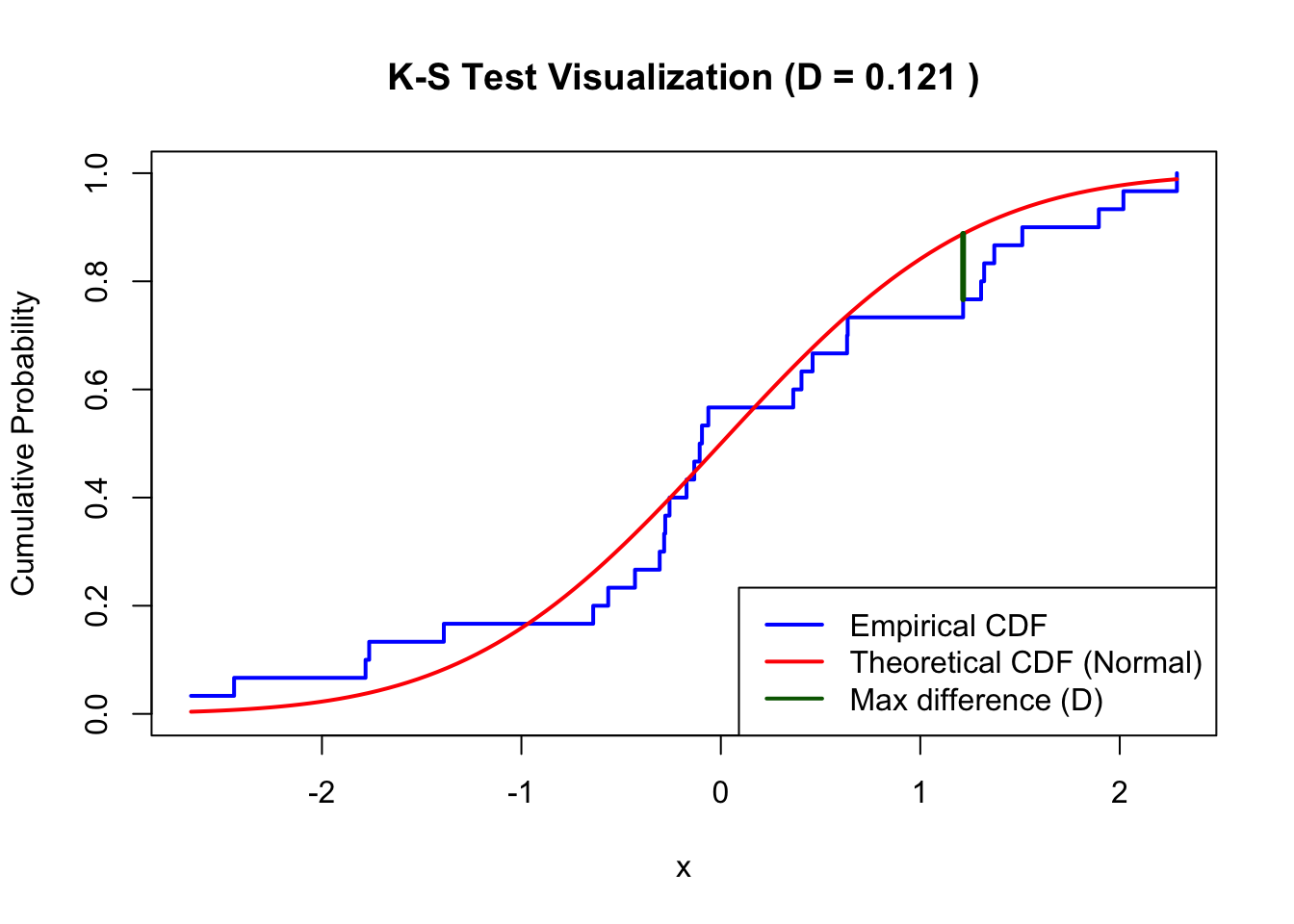
The K-S test statistic can be visualized as the maximum vertical distance between the empirical and theoretical CDFs:
Code
set.seed(42)x <-rnorm(30, mean =0, sd =1)# Compute ECDFecdf_x <-ecdf(x)x_sorted <-sort(x)ecdf_values <-ecdf_x(x_sorted)theoretical_values <-pnorm(x_sorted, mean =0, sd =1)# Find maximum differencedifferences <-abs(ecdf_values - theoretical_values)max_idx <-which.max(differences)D_stat <-max(differences)# Plotplot(x_sorted, ecdf_values, type ="s", lwd =2, col ="blue",xlab ="x", ylab ="Cumulative Probability",main =paste("K-S Test Visualization (D =", round(D_stat, 3), ")"),ylim =c(0, 1))curve(pnorm(x, mean =0, sd =1), add =TRUE, col ="red", lwd =2)# Draw maximum differencesegments(x_sorted[max_idx], ecdf_values[max_idx], x_sorted[max_idx], theoretical_values[max_idx],col ="darkgreen", lwd =3)legend("bottomright",legend =c("Empirical CDF", "Theoretical CDF (Normal)", "Max difference (D)"),col =c("blue", "red", "darkgreen"), lwd =2)
Figure 125.1: Visualization of K-S test statistic as maximum distance between ECDFs
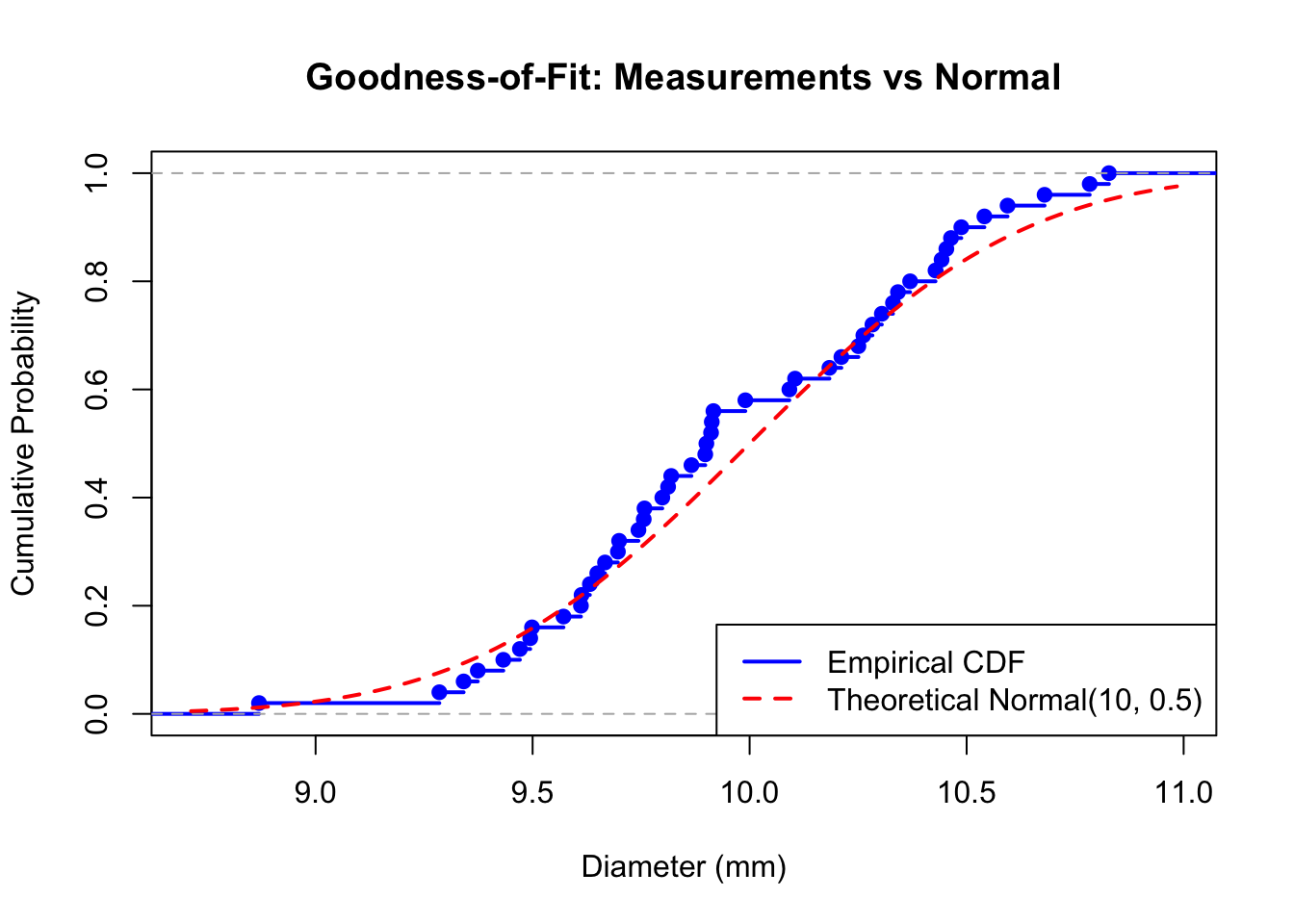
125.7 Example: Testing for Normality
A quality control engineer measures the diameter of 50 manufactured parts and wants to test if the measurements follow a normal distribution with mean 10mm and standard deviation 0.5mm:
# Simulated measurement data (slightly non-normal)set.seed(789)measurements <-c(rnorm(40, mean =10, sd =0.5),rnorm(10, mean =10.3, sd =0.3))# Test against specified normal distributionresult <-ks.test(measurements, "pnorm", mean =10, sd =0.5)print(result)# Summary statisticscat("\nSample mean:", round(mean(measurements), 3), "\n")cat("Sample SD:", round(sd(measurements), 3), "\n")
    Exact one-sample Kolmogorov-Smirnov test

data:  measurements
D = 0.12623, p-value = 0.3718
alternative hypothesis: two-sided


Sample mean: 9.968
Sample SD: 0.435
Code
# Visualizationplot(ecdf(measurements), main ="Goodness-of-Fit: Measurements vs Normal",xlab ="Diameter (mm)", ylab ="Cumulative Probability",col ="blue", lwd =2)curve(pnorm(x, mean =10, sd =0.5), add =TRUE, col ="red", lwd =2, lty =2)legend("bottomright",legend =c("Empirical CDF", "Theoretical Normal(10, 0.5)"),col =c("blue", "red"), lwd =2, lty =c(1, 2))
Figure 125.2: ECDF of measurements compared to theoretical normal distribution
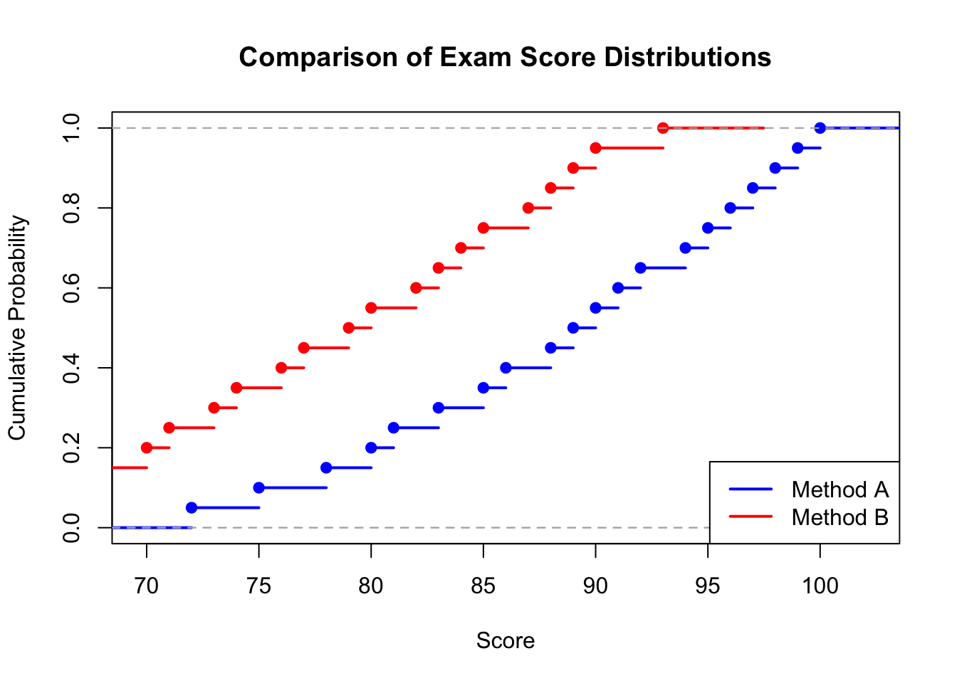
125.8 Example: Comparing Two Samples
A researcher wants to test if exam scores from two different teaching methods come from the same distribution:
    Exact two-sample Kolmogorov-Smirnov test

data:  method_A and method_B
D = 0.4, p-value = 0.07454
alternative hypothesis: two-sided
Code
# Plot both ECDFsplot(ecdf(method_A), col ="blue", lwd =2,main ="Comparison of Exam Score Distributions",xlab ="Score", ylab ="Cumulative Probability")plot(ecdf(method_B), add =TRUE, col ="red", lwd =2)legend("bottomright",legend =c("Method A", "Method B"),col =c("blue", "red"), lwd =2)
Figure 125.3: Comparison of ECDFs for two teaching methods
The small p-value indicates that the score distributions differ significantly between the two teaching methods.
125.9 Lilliefors Test
When testing for normality with parameters estimated from the data (rather than specified in advance), the standard K-S test is too conservative. The Lilliefors test (Lilliefors 1967) corrects for this:
# Install nortest package if neededinstall.packages("nortest")
# Test normality with estimated parametersset.seed(42)data <-rnorm(100, mean =50, sd =10)# Lilliefors test (uses estimated mean and SD)if (requireNamespace("nortest", quietly =TRUE)) { nortest::lillie.test(data)} else {cat("Install the 'nortest' package to run the Lilliefors test\n")}# Compare with standard K-S using estimated parameters (conservative)ks.test(data, "pnorm", mean =mean(data), sd =sd(data))
    Lilliefors (Kolmogorov-Smirnov) normality test

data:  data
D = 0.055683, p-value = 0.6253


    Asymptotic one-sample Kolmogorov-Smirnov test

data:  data
D = 0.055683, p-value = 0.9158
alternative hypothesis: two-sided
Note that the Lilliefors test gives a smaller p-value because it correctly accounts for parameter estimation.
125.10 Shapiro-Wilk Test
The Shapiro-Wilk test (Shapiro and Wilk 1965) is widely regarded as the most powerful test for normality, especially for small to moderate sample sizes (\(n < 50\)). It is specifically designed for testing whether data come from a normal distribution, unlike the K-S test which is a general-purpose goodness-of-fit test.
125.10.1 How It Works
The test statistic \(W\) is based on the correlation between the data and the expected normal order statistics:
\[
W = \frac{\left(\sum_{i=1}^{n} a_i x_{(i)}\right)^2}{\sum_{i=1}^{n} (x_i - \bar{x})^2}
\]
where \(x_{(i)}\) are the ordered sample values, \(\bar{x}\) is the sample mean, and \(a_i\) are constants derived from the means, variances, and covariances of the order statistics of a sample of size \(n\) from a standard normal distribution.
Intuitively, \(W\) measures how well the ordered data values match what we would expect from a normal distribution. Values of \(W\) close to 1 indicate normality; values significantly less than 1 indicate departure from normality.
125.10.2 Hypotheses
\[
H_0: \text{The data are normally distributed}
\]
\[
H_A: \text{The data are not normally distributed}
\]
125.10.3 R Code
The Shapiro-Wilk test is available in base R without any additional packages:
# Example 1: Normal dataset.seed(42)normal_data <-rnorm(50, mean =100, sd =15)cat("Test on normally distributed data:\n")shapiro.test(normal_data)
Test on normally distributed data:

    Shapiro-Wilk normality test

data:  normal_data
W = 0.98021, p-value = 0.5611
# Example 2: Non-normal data (exponential)set.seed(42)skewed_data <-rexp(50, rate =0.1)cat("Test on exponentially distributed data:\n")shapiro.test(skewed_data)
Test on exponentially distributed data:

    Shapiro-Wilk normality test

data:  skewed_data
W = 0.68815, p-value = 5.102e-09
The first test (normal data) yields a large p-value, so we do not reject normality. The second test (exponential data) yields a very small p-value, providing strong evidence against normality.
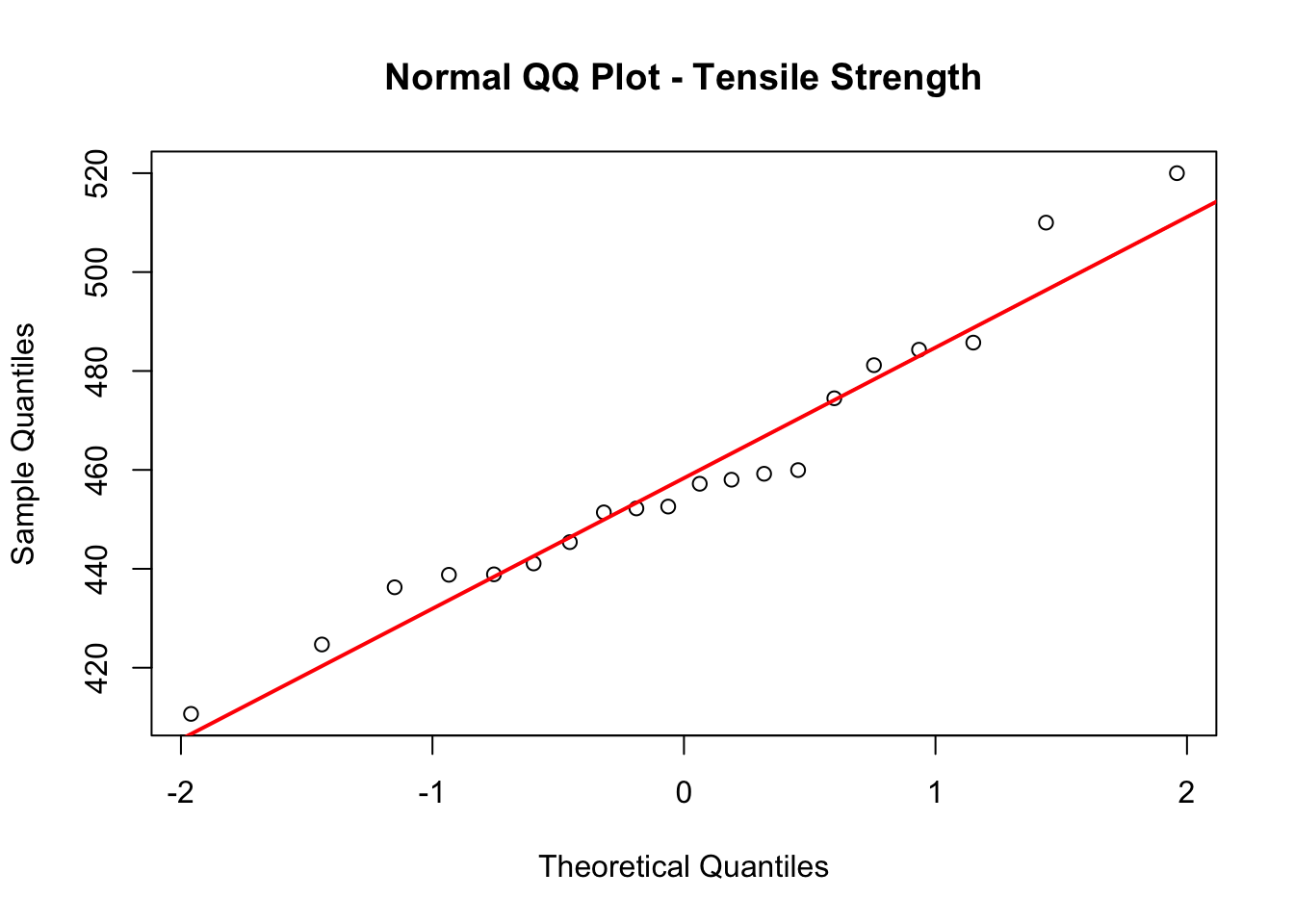
125.10.4 Worked Example
A manufacturer measures the tensile strength (in MPa) of 20 steel specimens and wants to verify that the measurements are normally distributed before applying a t-test:
qqnorm(strength, main ="Normal QQ Plot - Tensile Strength")qqline(strength, col ="red", lwd =2)
Figure 125.4: QQ plot of tensile strength data for visual normality assessment
125.10.5 Limitations
The sample size \(n\) must be between 3 and 5000
The test is sensitive to ties (repeated values); with many ties, the p-value may be unreliable
Like all hypothesis tests, the Shapiro-Wilk test becomes very sensitive with large samples – even trivial departures from normality may produce significant results when \(n\) is large
It tests only for normality, not for other distributions (unlike the K-S test)
125.10.6 Comparison: When to Use Which Normality Test
Table 125.3: Comparison of normality tests
Test
Best For
Limitations
R Function
Shapiro-Wilk
Small to moderate samples (\(n < 50\)); highest power
In practice, it is recommended to use the Shapiro-Wilk test as the primary formal test for normality, supplemented by a QQ plot for visual assessment.
125.11 Pros & Cons
125.11.1 Pros
The Kolmogorov-Smirnov test has the following advantages:
Does not require binning of continuous data, preserving all information.
Distribution-free for the two-sample case.
Works well with small sample sizes.
Sensitive to differences in location, scale, and shape of distributions.
Easy to visualize and interpret.
125.11.2 Cons
The Kolmogorov-Smirnov test has the following disadvantages:
For one-sample tests, parameters must be specified in advance (not estimated from data).
Less powerful than some alternatives (e.g., Anderson-Darling, Shapiro-Wilk for normality).
Most sensitive to differences near the center of the distribution, less sensitive in the tails.
Applies only to continuous distributions.
Ties in the data require special handling.
125.12 Related Tests
Anderson-Darling test: Similar to K-S but gives more weight to the tails of the distribution. Often more powerful for detecting departures from normality.
Shapiro-Wilk test: Specifically designed for testing normality; generally more powerful than K-S for this purpose.
Cramér-von Mises test: Uses the integral of the squared difference between CDFs rather than the maximum difference.
Chi-squared goodness-of-fit test (Section 124.1): Requires binning but can handle discrete distributions and estimated parameters.
125.13 Task
Generate 100 random numbers from an exponential distribution with rate \(\lambda = 0.5\). Use the K-S test to verify that the data follow this distribution.
Generate two samples: one from a standard normal distribution and one from a t-distribution with 5 degrees of freedom. Use the two-sample K-S test to determine if they differ significantly.
The following data represent waiting times (in minutes) at a service counter: 2.1, 0.5, 3.2, 1.8, 4.5, 0.9, 2.7, 1.2, 5.1, 0.3. Test whether these data follow an exponential distribution with mean 2 minutes.
Compare the K-S test and Chi-squared goodness-of-fit test on the same dataset. Discuss the advantages and disadvantages of each approach.
Kolmogorov, Andrey N. 1933. “Sulla Determinazione Empirica Di Una Legge Di Distribuzione.”Giornale Dell’Istituto Italiano Degli Attuari 4: 83–91.
Lilliefors, Hubert W. 1967. “On the Kolmogorov-Smirnov Test for Normality with Mean and Variance Unknown.”Journal of the American Statistical Association 62 (318): 399–402. https://doi.org/10.1080/01621459.1967.10482916.
Shapiro, S. S., and M. B. Wilk. 1965. “An Analysis of Variance Test for Normality (Complete Samples).”Biometrika 52 (3/4): 591–611. https://doi.org/10.1093/biomet/52.3-4.591.
Smirnov, Nickolay. 1948. “Table for Estimating the Goodness of Fit of Empirical Distributions.”The Annals of Mathematical Statistics 19 (2): 279–81. https://doi.org/10.1214/aoms/1177730256.