The Rayleigh distribution describes the magnitude (length) of a two-dimensional vector whose components are independent zero-mean Gaussian random variables. It is the standard model for signal envelope in wireless communications and for wind speed distributions.
Formally, the random variate \(X\) defined for the range \(X \in [0, \infty)\), is said to have a Rayleigh Distribution (i.e. \(X \sim \text{Rayleigh}(\sigma)\)) with scale parameter \(\sigma > 0\). If \(X_1, X_2 \overset{\text{i.i.d.}}{\sim} N(0, \sigma^2)\) then \(\sqrt{X_1^2 + X_2^2} \sim \text{Rayleigh}(\sigma)\).
34.1 Probability Density Function
\[
f(x) = \frac{x}{\sigma^2}\exp\!\left(-\frac{x^2}{2\sigma^2}\right), \quad x \geq 0
\]
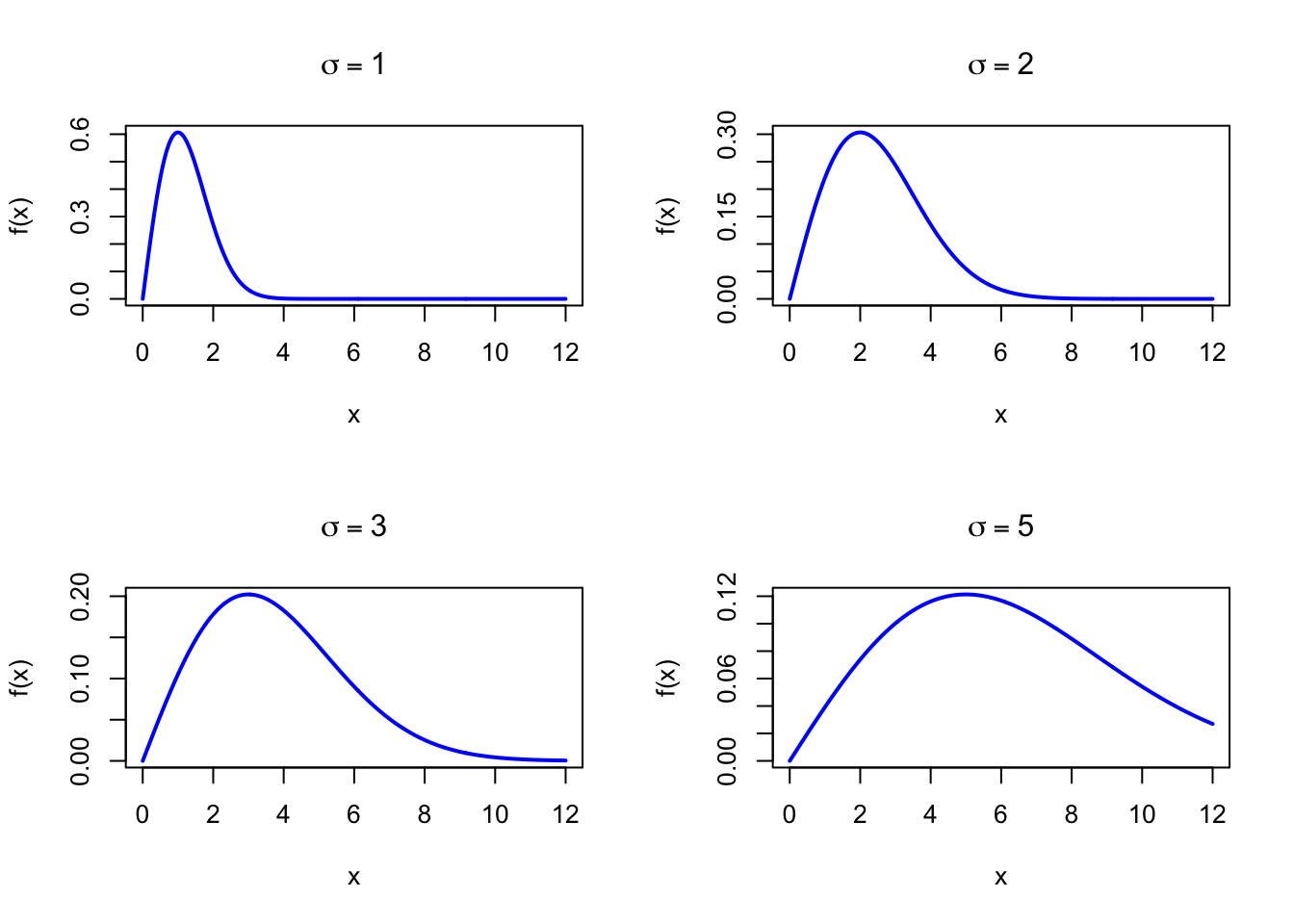
The figure below shows examples of the Rayleigh Probability Density Function for different scale values.
Code
drayleigh <-function(x, sigma) {ifelse(x >=0, x / sigma^2*exp(-x^2/ (2* sigma^2)), 0)}par(mfrow =c(2, 2))x <-seq(0, 12, length =500)plot(x, drayleigh(x, 1), type ="l", lwd =2, col ="blue",xlab ="x", ylab ="f(x)", main =expression(sigma ==1))plot(x, drayleigh(x, 2), type ="l", lwd =2, col ="blue",xlab ="x", ylab ="f(x)", main =expression(sigma ==2))plot(x, drayleigh(x, 3), type ="l", lwd =2, col ="blue",xlab ="x", ylab ="f(x)", main =expression(sigma ==3))plot(x, drayleigh(x, 5), type ="l", lwd =2, col ="blue",xlab ="x", ylab ="f(x)", main =expression(sigma ==5))par(mfrow =c(1, 1))
Figure 34.1: Rayleigh Probability Density Function for various scale values
34.2 Purpose
The Rayleigh distribution models the Euclidean magnitude of a 2D random vector with independent, equal-variance Gaussian components. Its elegant mathematical form and connection to the Normal distribution make it ideal for modeling magnitude quantities in physics, engineering, and communications. Common applications include:
Wireless communications: envelope of a narrowband signal with Rayleigh fading
Wind energy: marginal distribution of wind speed for power generation modeling
Underwater acoustics: noise envelope in sonar systems
Optics: speckle patterns in laser imaging
Navigation: radial positioning error from two independent Gaussian components
Relation to the discrete setting. The Rayleigh distribution models continuous 2D Euclidean magnitude; the closest discrete analog is a 2D random walk return distance. Conceptually related to the Geometric distribution as both model “distance” to first event in their respective spaces.
Wind speeds at a coastal site are modeled as \(X \sim \text{Rayleigh}(\sigma = 5)\) m/s. The mean wind speed is \(\sigma\sqrt{\pi/2} \approx 6.27\) m/s. We compute the probability of a gust exceeding 10 m/s.
This is a universal constant, independent of \(\sigma\).
34.25 Related Distributions 1: Weibull Distribution
The Rayleigh is a special case of the Weibull with shape \(k = 2\) (see Chapter 31).
34.26 Related Distributions 2: Chi Distribution
The Rayleigh distribution is the Chi distribution with 2 degrees of freedom, scaled by \(\sigma\): \(\text{Rayleigh}(\sigma) = \sigma \cdot \chi(2)\) (see Chapter 22).
34.27 Related Distributions 3: Maxwell-Boltzmann Distribution
The Maxwell-Boltzmann distribution is the three-dimensional analogue of the Rayleigh: while Rayleigh models the magnitude of a 2D Gaussian vector (\(k = 2\)), Maxwell-Boltzmann models the magnitude of a 3D Gaussian vector (\(k = 3\)). Both are special cases of the Chi distribution family (see Chapter 50).