155  Cross-Correlation Function

So far, the Box-Jenkins methodology has focused on a single time series: modelling its own past to generate forecasts. But many practical questions involve two series: does one series influence another, and if so, with what delay?

This chapter introduces the Cross-Correlation Function (CCF), which measures the linear association between two time series at different lags, and Granger causality, which formally tests whether one series helps predict another.

155.1 From Univariate to Bivariate

In Chapter 131 we studied the Pearson correlation between two variables measured at the same time. For time series, a static correlation is insufficient because the relationship between two series may involve a time delay: changes in series \(X\) may take several periods before they affect series \(Y\).

Consider the following example: when the price of Colombian coffee beans rises, how long does it take before US retail coffee prices adjust? The answer depends on shipping times, inventory buffers, and retail pricing decisions. The CCF allows us to identify this lead/lag structure empirically.

155.2 Definition

The cross-correlation function at lag \(k\) is defined as

\[ \rho_{XY}(k) = \text{Corr}(X_t, Y_{t+k}) = \frac{\gamma_{XY}(k)}{\sqrt{\gamma_{XX}(0) \cdot \gamma_{YY}(0)}} \]

where \(\gamma_{XY}(k) = \text{Cov}(X_t, Y_{t+k})\) is the cross-covariance at lag \(k\).

The interpretation of the sign of \(k\) is:

• Positive \(k\): \(X_t\) is correlated with \(Y_{t+k}\) — X leads Y by \(k\) periods
• Negative \(k\): \(X_t\) is correlated with \(Y_{t-|k|}\) — Y leads X by \(|k|\) periods

Unlike the autocorrelation function, the CCF is asymmetric: \(\rho_{XY}(k) \neq \rho_{XY}(-k)\) in general. This asymmetry is precisely what makes the CCF useful for identifying the direction of influence.

In R, the CCF is computed by ccf(x, y):

# Basic CCF computation
ccf(x, y, lag.max = 20, main = "Cross-Correlation Function")

Note

R’s ccf(x, y) plots \(\text{Corr}(X_{t+k}, Y_t)\) as a function of \(k\). A significant spike at negative lag \(k\) means \(X\) leads \(Y\) by \(|k|\) periods. Some textbooks use the opposite convention, so always check the documentation.

155.3 The Prewhitening Problem

155.3.1 Why Naive CCF Is Misleading

Computing the CCF directly on two raw time series is misleading whenever the series share common trends or have strong autocorrelation. Consider two series that both trend upward over time but have no causal relationship. The naive CCF will show large, significant cross-correlations at many lags — not because \(X\) influences \(Y\), but because both are driven by their own trends.

More formally, if \(X_t\) and \(Y_t\) are both autocorrelated, then \(X_t\) is correlated with \(X_{t-k}\) (by autocorrelation), and \(X_{t-k}\) may be spuriously correlated with \(Y_t\) (by shared trend). This inflates the CCF.

155.3.2 The Prewhitening Solution

To obtain a reliable CCF, we must remove the autocorrelation from both series using a technique called prewhitening:

Step 1: Fit an appropriate ARIMA model to \(X\) and extract the residuals \(\alpha_t\).

Step 2: Filter \(Y\) through the same ARIMA model (the one fitted to \(X\)) to obtain \(\beta_t\).

Step 3: Compute the CCF between \(\alpha_t\) and \(\beta_t\).

The key insight is that both series must be filtered through the same model — the one identified for \(X\) (Box and Jenkins 1970). This ensures that any remaining cross-correlation between \(\alpha_t\) and \(\beta_t\) reflects a genuine lead/lag relationship rather than shared autocorrelation structure.

# Prewhitening workflow
# Step 1: Fit ARIMA to X
fit_x <- arima(x, order = c(p, d, q))
alpha <- residuals(fit_x)

# Step 2: Filter Y through the same model
# Extract the AR and MA coefficients
beta <- residuals(arima(y, order = c(p, d, q),
                        fixed = coef(fit_x),
                        transform.pars = FALSE))

# Step 3: Compute CCF of prewhitened series
ccf(alpha, beta, main = "Prewhitened CCF")

155.4 Example: Coffee Prices

The coffee.csv dataset contains 360 monthly observations (30 years) of two series:

• Colombia: Colombian coffee import prices (input, \(X\))
• USA: US retail coffee prices (output, \(Y\))

The hypothesis is that changes in Colombian import prices lead US retail prices with some delay, due to shipping, inventory, and retail pricing adjustments.

coffee <- read.csv("coffee.csv")
colombia <- ts(coffee$Colombia, frequency = 12)
usa <- ts(coffee$USA, frequency = 12)

par(mfrow = c(2, 1), mar = c(4, 4, 3, 1))
plot(colombia, lwd = 2, col = "steelblue",
     main = "Colombia Import Price", ylab = "Price")
plot(usa, lwd = 2, col = "coral",
     main = "USA Retail Price", ylab = "Price")
par(mfrow = c(1, 1))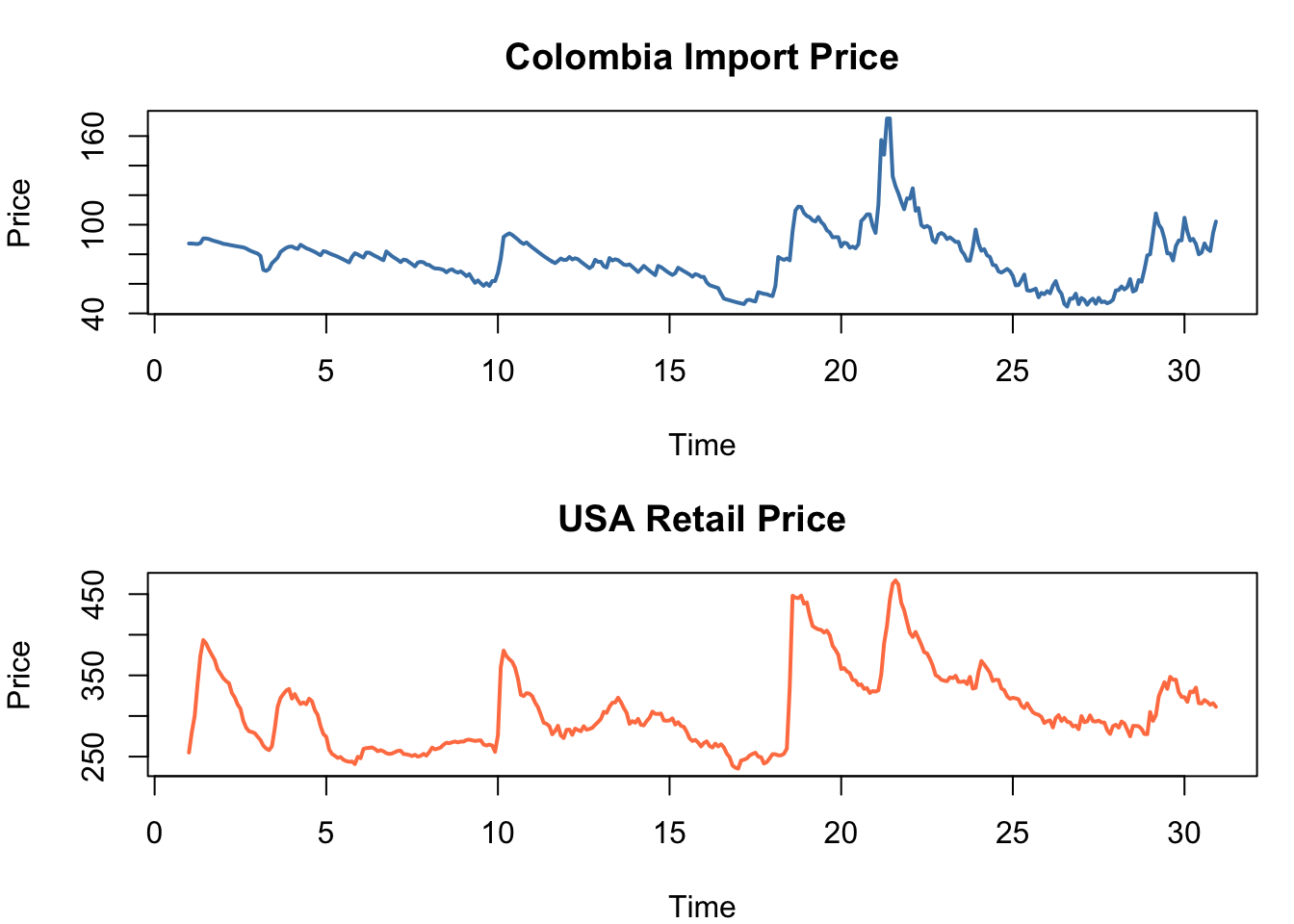

Figure 155.1: Colombian import and US retail coffee prices

155.4.1 Naive CCF (Misleading)

ccf(as.numeric(colombia), as.numeric(usa), lag.max = 24,
    main = "Naive CCF: Colombia vs USA Coffee Prices",
    xlab = "Lag", ylab = "CCF")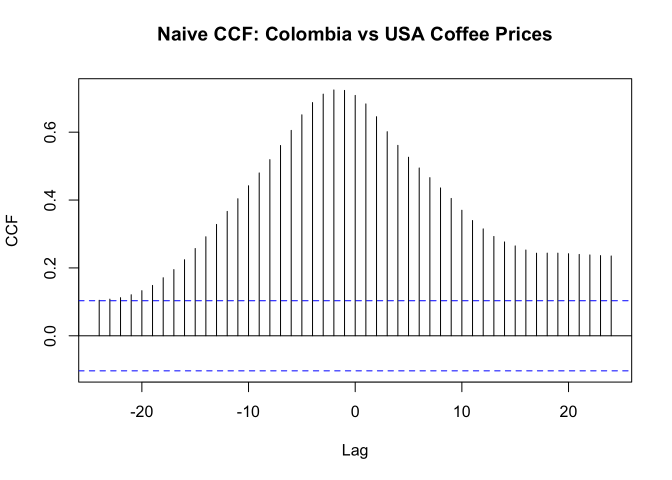

Figure 155.2: Naive CCF between coffee prices (misleading due to shared trends)

The naive CCF shows large positive correlations at many lags. This is expected — both series trend together — but it does not reveal the true lead/lag structure.

155.4.2 Prewhitened CCF

# Step 1: Fit ARIMA to Colombia (input)
col_diff <- diff(colombia)
usa_diff <- diff(usa)
fit_col_d <- arima(col_diff, order = c(1, 0, 1))
alpha_d <- residuals(fit_col_d)

# Step 2: Filter USA through the same model
beta_d <- residuals(arima(usa_diff, order = c(1, 0, 1),
                          fixed = coef(fit_col_d),
                          transform.pars = FALSE))

# Keep only aligned complete observations
pw <- data.frame(alpha = as.numeric(alpha_d), beta = as.numeric(beta_d))
pw <- pw[complete.cases(pw), ]

ccf(pw$alpha, pw$beta,
    lag.max = 24,
    main = "Prewhitened CCF: Colombia vs USA Coffee Prices",
    xlab = "Lag", ylab = "CCF")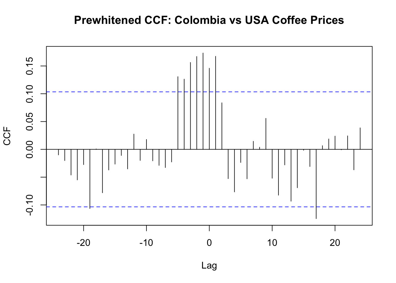

Figure 155.3: Prewhitened CCF between coffee prices

The prewhitened CCF reveals the true cross-correlation structure, stripped of confounding autocorrelation. The dominant pattern is at negative lags: several significant spikes confirm that Colombia import prices lead US retail prices, consistent with the expected supply-chain pass-through (shipping, inventory, retail repricing).

However, a secondary significant spike also appears at k = 1, suggesting that current US retail prices contain information about next month’s Colombia import prices. This opposite-side spike may reflect:

• anticipation — retailers observe futures markets or contract negotiations and adjust shelf prices before the official import price index moves,
• publication timing — the import and retail price indices may be compiled on slightly different schedules, creating an apparent lead that is really a measurement artefact, or
• residual confounding — imperfect prewhitening may leave trace autocorrelation that inflates a single lag.

A single significant spike on the opposite side does not, by itself, prove structural anticipation. But it does suggest that the Colombia → USA relationship may not be purely unidirectional. If the bidirectional pattern persists after robustness checks (e.g. varying ARIMA orders or lag truncation), a feedback framework such as VAR or ECM/VECM (Section 157.3) may be more appropriate than a one-way transfer function model.

Note

The dedicated CCF app is available at https://shiny.wessa.net/CCFPrewhiten/ (RFC menu item: Time Series / Cross Correlation Function).

Interactive Shiny app (click to load).

Open in new tab

155.5 Interpreting the CCF

The prewhitened CCF is used to identify the parameters of the transfer function model (Chapter 156). The pattern of significant spikes suggests the delay (\(b\)), the order of the numerator (\(s\)), and the order of the denominator (\(r\)) of the transfer function.

Table 155.1: CCF patterns and implied transfer function structures

CCF pattern	Implied TF structure
Single spike at lag \(b\)	\(v(B) = \omega_0 B^b\) (simple delay, no dynamics)
Spike at lag \(b\) followed by exponential decay	\(v(B) = \frac{\omega_0}{1 - \delta_1 B} B^b\) (first-order denominator)
Spikes at lags \(b\) and \(b+1\), then zero	\(v(B) = (\omega_0 - \omega_1 B) B^b\) (first-order numerator)
Spikes starting at lag \(b\) with slow decay	Higher-order transfer function

The delay parameter \(b\) corresponds to the first lag at which a significant spike appears in the prewhitened CCF. The shape of the decay after lag \(b\) determines whether the transfer function has AR-like dynamics (\(r > 0\)) or a finite impulse response (\(r = 0\)).

155.6 Granger Causality

While the CCF is a descriptive measure of lead/lag association, Granger causality (Granger 1969) provides a formal statistical test. The question it answers is:

Does the past of \(X\) improve the prediction of \(Y\) beyond the past of \(Y\) alone?

If yes, we say that \(X\) Granger-causes \(Y\).

155.6.1 Definition

The Granger causality test compares two models:

Restricted model (only own lags):

\[ Y_t = \alpha + \sum_{i=1}^{p} \beta_i Y_{t-i} + e_t \]

Unrestricted model (own lags + lags of X):

\[ Y_t = \alpha + \sum_{i=1}^{p} \beta_i Y_{t-i} + \sum_{j=1}^{p} \gamma_j X_{t-j} + u_t \]

The null hypothesis is \(H_0: \gamma_1 = \gamma_2 = \ldots = \gamma_p = 0\) (X does not Granger-cause Y). The test statistic is an F-test (or Wald test) comparing the two models.

Before applying Granger tests, use this decision rule:

1. If both series are stationary, test in levels.
2. If both are non-stationary and not cointegrated, difference first and test on differenced series.
3. If both are non-stationary and cointegrated, use an ECM/VECM framework instead of a plain levels test.

155.6.2 Important caveat

“Granger causality” is a statistical concept, not a philosophical one. It means predictive precedence, not true causation. A variable can Granger-cause another because:

• It truly causes it
• Both are caused by a third variable, with different delays
• The relationship is a statistical artefact

As discussed in Chapter 132, establishing true causality requires additional reasoning beyond statistical tests.

155.6.3 Example: Coffee Prices

Before applying the Granger test we verify the integration order of both series using the augmented Dickey-Fuller (ADF) unit-root test (Dickey and Fuller 1979). As noted in the decision rule above, levels Granger testing requires stationarity of both series; if either is integrated, either difference both (when not cointegrated) or apply an ECM/VECM (when cointegrated).

# Granger causality test using lmtest package
library(lmtest)
library(tseries)

coffee <- read.csv("coffee.csv")
colombia <- ts(coffee$Colombia, frequency = 12)
usa <- ts(coffee$USA, frequency = 12)

# Quick stationarity check (illustrative)
cat("ADF test (levels): Colombia p-value =", adf.test(as.numeric(colombia))$p.value, "\n")
cat("ADF test (levels): USA p-value =", adf.test(as.numeric(usa))$p.value, "\n\n")

# For this example we proceed on first differences
dy <- diff(as.numeric(usa))
dx <- diff(as.numeric(colombia))
gr_data <- data.frame(dy = dy, dx = dx)

cat("Test 1 (differenced data): Does Colombia Granger-cause USA?\n")
g1 <- grangertest(dy ~ dx, order = 6, data = gr_data)
print(g1)

cat("\nTest 2 (differenced data): Does USA Granger-cause Colombia?\n")
g2 <- grangertest(dx ~ dy, order = 6, data = gr_data)
print(g2)

cat("\nInterpretation guide:\n")
cat("- p-value < 0.05: reject H0, lagged predictor adds forecasting information.\n")
cat("- p-value >= 0.05: do not reject H0 at the 5% level.\n")

ADF test (levels): Colombia p-value = 0.252716 
ADF test (levels): USA p-value = 0.03955398 

Test 1 (differenced data): Does Colombia Granger-cause USA?
Granger causality test

Model 1: dy ~ Lags(dy, 1:6) + Lags(dx, 1:6)
Model 2: dy ~ Lags(dy, 1:6)
  Res.Df Df      F    Pr(>F)    
1    340                        
2    346 -6 5.1475 4.416e-05 ***
---
Signif. codes:  0 '***' 0.001 '**' 0.01 '*' 0.05 '.' 0.1 ' ' 1

Test 2 (differenced data): Does USA Granger-cause Colombia?
Granger causality test

Model 1: dx ~ Lags(dx, 1:6) + Lags(dy, 1:6)
Model 2: dx ~ Lags(dx, 1:6)
  Res.Df Df     F   Pr(>F)   
1    340                     
2    346 -6 3.465 0.002451 **
---
Signif. codes:  0 '***' 0.001 '**' 0.01 '*' 0.05 '.' 0.1 ' ' 1

Interpretation guide:
- p-value < 0.05: reject H0, lagged predictor adds forecasting information.
- p-value >= 0.05: do not reject H0 at the 5% level.

The results indicate whether the relationship is unidirectional (Colombia leads USA only) or bidirectional. In this context, unidirectional Granger causality from Colombia to USA is economically plausible because production/import prices tend to lead retail pricing decisions.

155.6.4 Interactive Granger App

The dedicated Granger app is available at https://shiny.wessa.net/Granger/ (RFC menu item: Time Series / Granger Causality).

Compared with the basic R example above, the app adds practical controls that are important for robustness:

• separate differencing settings for \(Y\) and \(X\),
• lag order selection \(p\),
• a delay parameter \(b\) (default 0) so the predictor block is tested on lags \((b+1)\) to \((b+p)\),
• a robustness grid with an Apply button to refit immediately from a selected grid row.

Interactive Shiny app (click to load).

Open in new tab

155.7 Tasks

1. Compute the naive and prewhitened CCF for the Coffee series. How do the two plots differ? Which lags are significant in the prewhitened version but not in the naive version, and vice versa?

2. Test Granger causality in both directions (Colombia \(\rightarrow\) USA and USA \(\rightarrow\) Colombia). Is the relationship unidirectional? Experiment with different lag orders (e.g. 3, 6, 12).

3. Vary the maximum lag in the Granger test (the order parameter). Does the conclusion change with the number of lags? What does this suggest about the appropriate lag length?

Box, George E. P., and Gwilym M. Jenkins. 1970. Time Series Analysis: Forecasting and Control. San Francisco: Holden-Day.

Dickey, David A., and Wayne A. Fuller. 1979. “Distribution of the Estimators for Autoregressive Time Series with a Unit Root.” Journal of the American Statistical Association 74 (366): 427–31. https://doi.org/10.1080/01621459.1979.10482531.

Granger, Clive W. J. 1969. “Investigating Causal Relations by Econometric Models and Cross-Spectral Methods.” Econometrica 37 (3): 424–38. https://doi.org/10.2307/1912791.