26  Fisher F-Distribution

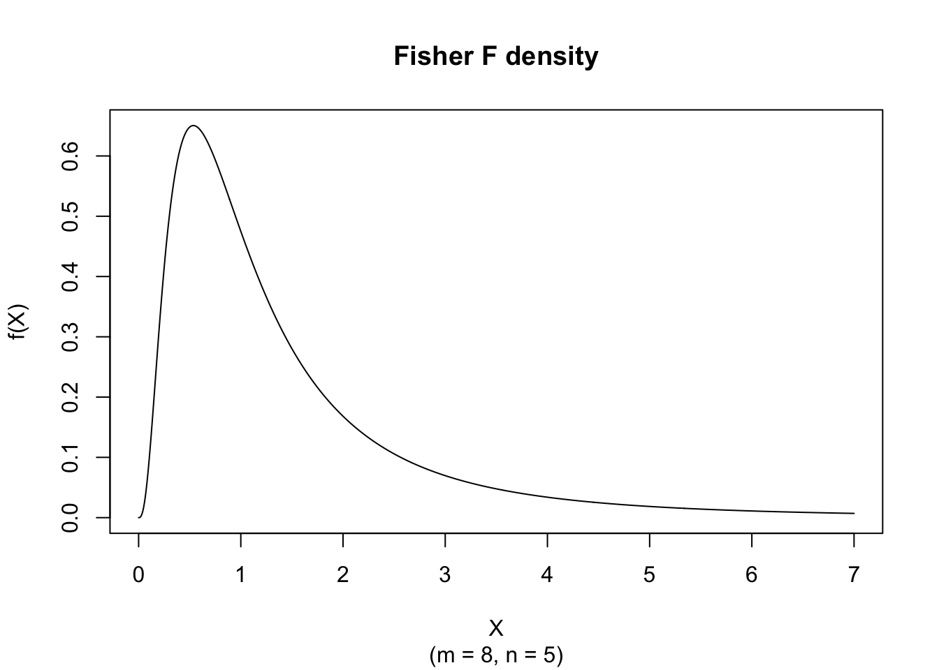
The random variate \(X\) defined for the range \(0 \leq X \leq +\infty\), is said to have an F-Distribution (i.e. \(X \sim \text{F} \left( m, n \right)\)) with shape parameters \(m, n \in \mathbb{N}^+\).

26.1 Probability Density Function

\[ f(X) = \frac{\left( \frac{m}{n} \right)^{\frac{m}{2}} X^{\frac{m}{2}-1} }{\text{B} \left[ \frac{m}{2}, \frac{n}{2} \right] \left[ 1 + \left( \frac{m}{n} \right) X \right]^{\frac{m+n}{2}} } \]

The figure below shows an example of the Fisher Probability Density function with \(m = 8\) and \(n = 5\).

x <- seq(0,7,length=1000)
hx <- df(x, df1 = 8, df2 = 5)
plot(x, hx, type="l", xlab="X", ylab="f(X)", xlim=c(0,7), main="Fisher F density", sub = "(m = 8, n = 5)")

Figure 26.1: Example of Fisher Probability Density Function (m = 8, n = 5)

26.2 Distribution Function

There is no elementary closed form of the Distribution Function; it is expressed exactly via the regularized incomplete beta function and computed by pf().

26.3 Uncentered Moments

\[ \mu_j' = \left( \frac{n}{m} \right)^j \frac{\Gamma \left[ \frac{m}{2} + j \right] \Gamma \left[ \frac{n}{2} -j \right] }{\Gamma \left[ \frac{m}{2} \right] \Gamma \left[ \frac{n}{2} \right] } \]

for \(n > 2 j\).

26.4 Expected Value

\[ \text{E}(X) = \frac{n}{n-2} \]

for \(n > 2\).

26.5 Variance

\[ \text{V}(X) = \frac{2n^2 (m+n-2)}{m(n-2)^2(n-4)} \]

for \(n > 4\).

26.6 Mode

\[ \text{Mo}(X) = \frac{n}{m} \frac{m-2}{n+2} \]

for \(m > 2\).

26.7 Skewness

\[ g_1 = \frac{(2m + n -2)}{(n-6)} \sqrt{\frac{8(n-4)}{m(m+n-2)}} \]

for \(n > 6\).

26.8 Kurtosis

\[ g_2 = 3 + \frac{12 \left[m(5n-22)(m+n-2) + (n-4)(n-2)^2\right]}{m(n-6)(n-8)(m+n-2)} \]

for \(n > 8\).

26.9 Coefficient of Variation

\[ VC = \sqrt{\frac{2(m+n-2)}{m(n-4)}} \]

for \(n > 4\).

26.10 Random Number Generator

Random numbers from the F variate with \(m\) and \(n\) degrees of freedom, denoted by F\((m,n)\), can be computed by using the relationship between the F variate and two independent Chi-squared variates.

Let

\[ \begin{cases} \chi^2(m) \text{ denote a Chi-squared variate with m degrees of freedom} \\ \chi^2(n) \text{ denote a Chi-squared variate with n degrees of freedom} \\ \text{N}(0,1) \text{ denote a unit normal variate} \end{cases} \]

then

\[ \text{F}(m,n) \sim \frac{\frac{1}{m} \sum_{i=1}^{m}\text{N}_i(0,1)^2}{\frac{1}{n}\sum_{i=1}^{n}\text{N}_i(0,1)^2} = \frac{\frac{\chi^2(m)}{m}}{\frac{\chi^2(n)}{n}} \]

26.11 Properties 1: Mean Depends Only on Second df

The first parameter, \(m\), does not affect the expected value.

26.12 Properties 2: Large-df Normal Approximation (After Scaling)

As the degrees of freedom \(m\) and \(n\) increase, a suitably centered and scaled F\((m,n)\) variate approaches normality.

26.13 Properties 3: Reciprocal Symmetry

The inverse of an F variate with \(m\) and \(n\) degrees of freedom, denoted by F\((m,n)\), is also an F variate but with degrees of freedom \(n\) and \(m\), i.e.

\[ \text{F}(n,m) \sim \frac{1}{\text{F}(m,n)} \]

26.14 Related Distributions 1: Beta-tail Identity

The Beta variate with shape parameters \(\frac{m}{2}\) and \(\frac{n}{2}\), denoted by B\((\frac{m}{2}, \frac{n}{2})\), and the Fisher F variate with \(m\) and \(n\) degrees of freedom, denoted by F\((m,n)\), are related:

\[ \text{P} \left[ \text{B} \left( \frac{m}{2}, \frac{n}{2} \right) \leq \frac{m}{m + n X} \right] = \text{P} \left[ \text{F} (m,n) \geq X \right] \]

26.15 Related Distributions 2: Transforming Beta to F (Y/(1-Y))

If \(Y \sim \text{B}(m,n)\) then \(X = \frac{n}{m} \frac{Y}{1-Y} \sim \text{F}(2m, 2n)\).

26.16 Related Distributions 3: Transforming Beta to F ((1-Y)/Y)

If \(Y \sim \text{B}(m,n)\) then \(X = \frac{m}{n} \frac{1-Y}{Y} \sim \text{F}(2n, 2m)\).

26.17 Related Distributions 4: Transforming F to Beta (Reciprocal Form)

If \(Y \sim \text{F}(m,n)\) then \(X = \frac{1}{1 + \frac{m}{n} Y} \sim \text{B} \left( \frac{n}{2}, \frac{m}{2} \right)\).

26.18 Related Distributions 5: Transforming F to Beta (Direct Form)

If \(Y \sim \text{F}(m,n)\) then \(X = \frac{\frac{m}{n} Y }{1 + \frac{m}{n} Y} \sim \text{B} \left( \frac{m}{2}, \frac{n}{2} \right)\).

26.19 Related Distributions 6: Ratio of Chi-squared Variables

The Chi-squared variate with \(m\) degrees of freedom, denoted by \(\chi^2(m)\), and the Chi-squared variate with \(n\) degrees of freedom, denoted \(\chi^2(n)\), are related to the F variate with \(m\) and \(n\) degrees of freedom:

\[ \text{F}(m,n) \sim \frac{\frac{\chi^2(m)}{m}}{\frac{\chi^2(n)}{n}} \]

26.20 Related Distributions 7: Chi-squared as Limit of F

The Chi-squared variate with \(m\) degrees of freedom is equal to \(m\) times the F variate with degrees of freedom equal to \(m\) and \(+\infty\), i.e.

\[ \chi^2(m) \sim m \times \text{F}(m, +\infty) \]

26.21 Related Distributions 8: Variance Ratio Using Biased Sample Variances

Consider two sets of normal variates, i.e.

\[ \text{N}_{ij} \left( \mu_i, \sigma_i^2 \right) \]

for \(i = 1, 2\) and \(j = 1, 2, …, n_i\).

In addition, let the variate \(\bar{x}\) and \(s_i^2\) be defined as

\[ \begin{cases} \bar{x} = \frac{1}{n_i} \sum_{j=1}^{n_i} \text{N}_{ij} \left( \mu_i, \sigma_i^2 \right) \\ s_i^2 = \frac{1}{n_i} \sum_{j=1}^{n_i} \left[ \text{N}_{ij} \left( \mu_i, \sigma_i^2 \right) - \bar{x} \right]^2 \end{cases} \]

then

\[ \text{F}(m,n) \sim \frac{\frac{\frac{n_1 s_1^2}{\sigma_1^2}}{m}}{\frac{\frac{n_2 s_2^2}{\sigma_2^2}}{n}} = \frac{\sigma_2^2}{\sigma_1^2} \frac{s_1^2}{s_2^2} \frac{n_1}{n_2} \frac{n_2 - 1}{n_1 - 1} \]

where \(m = (n_1 - 1)\) and \(n = (n_2 - 1)\).

Note that this section uses the biased variance definition with denominator \(n_i\).

26.22 Related Distributions 9: Variance Ratio Using Unbiased Sample Variances

Consider two sets of normal variates, i.e.

\[ \text{N}_{ij} \left( \mu_i, \sigma_i^2 \right) \]

for \(i = 1, 2\) and \(j = 1, 2, …, n_i\).

In addition, let the variate \(\bar{x}\) and \(s_i^2\) be defined as

\[ \begin{cases} \bar{x} = \frac{1}{n_i} \sum_{j=1}^{n_i} \text{N}_{ij} \left( \mu_i, \sigma_i^2 \right) \\ s_i^2 = \frac{1}{n_i-1} \sum_{j=1}^{n_i} \left[ \text{N}_{ij} \left( \mu_i, \sigma_i^2 \right) - \bar{x} \right]^2 \end{cases} \]

then

\[ \text{F}(m,n) \sim \frac{\frac{\frac{(n_1-1) s_1^2}{\sigma_1^2}}{n_1-1}}{\frac{\frac{(n_2-1) s_2^2}{\sigma_2^2}}{n_2-1}} = \frac{\sigma_2^2}{\sigma_1^2} \frac{s_1^2}{s_2^2} \]

where \(m = (n_1 - 1)\) and \(n = (n_2 - 1)\).

This section uses the unbiased variance definition with denominator \((n_i-1)\).

26.23 Related Distributions 10: Noncentral F Distribution

The noncentral \(F\) distribution generalises the Fisher \(F\) by adding a noncentrality parameter \(\lambda \neq 0\). It arises when performing ANOVA or regression \(F\)-tests under the alternative hypothesis, and is the primary tool for power analysis and sample-size planning for these tests (see Chapter 48).

26.24 Example

Suppose we compare two independent sample variances and obtain \(s_1^2/s_2^2 = 1.8\) with \((m,n)=(12,15)\). A right-tail probability is:

1 - pf(1.8, df1 = 12, df2 = 15)

[1] 0.1405509

26.25 Purpose

The F-distribution is central to variance-ratio inference, including ANOVA, regression F-tests, and model-comparison procedures based on nested sums of squares.