154  Intervention Analysis

In Chapter 153 we observed that the pure ARIMA model for the Soldiers time series produced a technically correct but practically useless forecast. The footnote noted that “the American President decided to withdraw US troops from Iraq” — a known event that fundamentally changed the level of the series. The ARIMA model could not capture this because it only uses the series’ own past to generate forecasts.

This chapter introduces intervention analysis (Box and Tiao 1975), a formal extension of the Box-Jenkins framework that incorporates known external events into the ARIMA model.

154.1 When Ceteris Paribus Fails

The ceteris paribus assumption underlying ARIMA forecasts states that no exceptional events occur during the forecast period. When this assumption is violated, the forecasting errors can be very large — not because the model is statistically wrong, but because the world changed in a way the model cannot account for.

Consider three cases from the earlier chapters:

• Soldiers: The troop withdrawal was a political decision, not a statistical pattern. The series dropped from roughly 80-100 KIA/month to single digits.
• Unemployment: Around the 2008 financial crisis, unemployment shows a sudden, persistent increase around observation 300.
• Seatbelts (new in this chapter): The UK Road Traffic Act mandated seatbelt use from January 1983, permanently reducing casualties.

In each case, a specific, identifiable event is plausibly associated with a structural break in the series. Intervention analysis allows us to model such events explicitly.

154.2 The Intervention Function

154.2.1 Pulse and Step Variables

An intervention is represented by an indicator variable \(I_t^{(T)}\) that marks the time \(T\) at which the event occurs. The two most common forms are:

Pulse intervention — a one-time shock at time \(T\):

\[ P_t^{(T)} = \begin{cases} 1 & \text{if } t = T \\ 0 & \text{otherwise} \end{cases} \]

Step intervention — a permanent level shift starting at time \(T\):

\[ S_t^{(T)} = \begin{cases} 1 & \text{if } t \geq T \\ 0 & \text{if } t < T \end{cases} \]

Note that the step variable is the cumulative sum of the pulse: \(S_t^{(T)} = \sum_{j=-\infty}^{t} P_j^{(T)}\). In the backshift operator notation, \(S_t^{(T)} = \frac{1}{1-B} P_t^{(T)}\).

154.2.2 Dynamic Response Patterns

The intervention function \(v(B)\) describes how the effect of the event unfolds over time. Combined with the intervention variable, the response is \(v(B) I_t^{(T)}\). Four common patterns are:

Table 154.1: Dynamic response patterns for intervention models

Pattern	Model	Interpretation
Abrupt, permanent	\(\omega_0 S_t^{(T)}\)	Immediate level shift that persists
Abrupt, temporary	\(\omega_0 P_t^{(T)}\)	One-time shock, series returns to baseline
Gradual, permanent	\(\frac{\omega_0}{1 - \delta_1 B} S_t^{(T)}\)	Gradual transition to new level
Gradual, temporary	\(\frac{\omega_0}{1 - \delta_1 B} P_t^{(T)}\)	Temporary effect that decays over time

The parameter \(\omega_0\) measures the magnitude of the intervention effect and \(\delta_1\) (with \(|\delta_1| < 1\)) controls the rate at which the effect builds up or decays.

par(mfrow = c(2, 2), mar = c(4, 4, 3, 1))
t <- 1:50
T0 <- 20
omega <- -50
delta <- 0.8

# Abrupt, permanent (step)
step <- ifelse(t >= T0, 1, 0)
y1 <- omega * step
plot(t, y1, type = "l", lwd = 2, col = "steelblue",
     main = "Abrupt, permanent", xlab = "t", ylab = "Effect")
abline(v = T0, lty = 2, col = "grey50")

# Abrupt, temporary (pulse)
pulse <- ifelse(t == T0, 1, 0)
y2 <- omega * pulse
plot(t, y2, type = "l", lwd = 2, col = "coral",
     main = "Abrupt, temporary", xlab = "t", ylab = "Effect")
abline(v = T0, lty = 2, col = "grey50")

# Gradual, permanent
y3 <- numeric(50)
for (i in T0:50) y3[i] <- omega * (1 - delta^(i - T0 + 1)) / (1 - delta)
plot(t, y3, type = "l", lwd = 2, col = "steelblue",
     main = "Gradual, permanent", xlab = "t", ylab = "Effect")
abline(v = T0, lty = 2, col = "grey50")

# Gradual, temporary
y4 <- numeric(50)
y4[T0] <- omega
for (i in (T0+1):50) y4[i] <- delta * y4[i-1]
plot(t, y4, type = "l", lwd = 2, col = "coral",
     main = "Gradual, temporary", xlab = "t", ylab = "Effect")
abline(v = T0, lty = 2, col = "grey50")

par(mfrow = c(1, 1))

Figure 154.1: Four dynamic response patterns to an intervention at t = 20

154.3 The Intervention Model

The full intervention model takes the form

\[ Y_t = v(B) I_t^{(T)} + N_t \]

where \(v(B) I_t^{(T)}\) is the deterministic intervention effect and \(N_t\) follows an ARIMA process — that is, \(N_t\) is the noise component that we already know how to model from the previous chapters. In the simplest case of an abrupt, permanent intervention:

\[ Y_t = \omega_0 S_t^{(T)} + N_t \]

This model separates the series into two parts: the effect of the known event (\(\omega_0 S_t^{(T)}\)) and the stochastic ARIMA dynamics (\(N_t\)). The \(N_t\) component is exactly the type of model developed in Chapter 151 through Chapter 153.

In R, this model is estimated using the arima() function with the xreg argument, which accepts a matrix of external regressors. Each column of xreg represents one intervention variable (pulse, step, or other external input).

Note

The ad hoc forecasting approach in Chapter 147 introduced intervention variables informally as regression dummies. This chapter formalises that idea within the Box-Jenkins framework, where the noise \(N_t\) is explicitly modelled as an ARIMA process rather than assumed to be white noise.

154.4 Example: UK Seatbelt Law

R’s built-in Seatbelts dataset contains monthly data on road casualties in the UK from January 1969 to December 1984 (192 observations). The Road Traffic Act mandated front-seat seatbelt use from January 1983, corresponding to observation \(t = 169\).

We use the DriversKilled variable as our target series and model the seatbelt law as a step intervention.

# Load the data
data(Seatbelts)
y <- Seatbelts[, "DriversKilled"]
y_ts <- ts(y, start = c(1969, 1), frequency = 12)

# Plot the series
plot(y_ts, lwd = 2, ylab = "Drivers Killed", xlab = "Year",
     main = "UK Drivers Killed (Monthly)")
abline(v = 1983 + 0/12, col = "red", lwd = 2, lty = 2)
text(1983.5, max(y) * 0.95, "Seatbelt law", col = "red", pos = 4)

Figure 154.2: UK drivers killed per month, with seatbelt law intervention point

The visual inspection suggests a clear drop in the level of the series after January 1983. We now fit an ARIMA model with a step intervention.

# Create the step intervention variable
n <- length(y)
step_law <- c(rep(0, 168), rep(1, n - 168))

# Fit ARIMA with intervention
# First, identify a suitable ARIMA order for the noise
# Based on the seasonal pattern and previous BJ analysis:
fit_intervention <- arima(y_ts,
                          order = c(1, 0, 0),
                          seasonal = list(order = c(1, 1, 1), period = 12),
                          xreg = step_law)
cat("ARIMA(1,0,0)(1,1,1)[12] with step intervention:\n")
print(fit_intervention)

ARIMA(1,0,0)(1,1,1)[12] with step intervention:

Call:
arima(x = y_ts, order = c(1, 0, 0), seasonal = list(order = c(1, 1, 1), period = 12), 
    xreg = step_law)

Coefficients:
         ar1    sar1     sma1  step_law
      0.4043  0.2237  -0.9454  -22.1932
s.e.  0.0721  0.1175   0.2012    6.7872

sigma^2 estimated as 248.6:  log likelihood = -761.81,  aic = 1533.61

# The coefficient of the step variable (xreg) estimates the
# change in monthly driver deaths associated with the law indicator
coefs <- coef(fit_intervention)
cat("\nEstimated intervention effect (omega_0):",
    round(coefs["step_law"], 1), "drivers killed per month\n")
cat("Standard error:", round(sqrt(fit_intervention$var.coef["step_law", "step_law"]), 1), "\n")

Estimated intervention effect (omega_0): -22.2 drivers killed per month
Standard error: 6.8 

The negative coefficient \(\hat{\omega}_0\) represents the estimated reduction in monthly driver fatalities associated with the seatbelt law indicator, controlling for ARIMA dynamics and seasonality.

# Residual diagnostics
par(mfrow = c(2, 2), mar = c(4, 4, 3, 1))
resid <- residuals(fit_intervention)
plot(resid, main = "Residuals over time", ylab = "Residual")
abline(h = 0, lty = 2)
acf(resid, main = "ACF of Residuals", na.action = na.pass)
pacf(resid, main = "PACF of Residuals", na.action = na.pass)
qqnorm(resid, main = "QQ Plot of Residuals")
qqline(resid, col = "red")
par(mfrow = c(1, 1))

# Ljung-Box test
cat("\nLjung-Box test on residuals:\n")
print(Box.test(resid, lag = 24, type = "Ljung-Box"))

Ljung-Box test on residuals:

    Box-Ljung test

data:  resid
X-squared = 41.098, df = 24, p-value = 0.01625

Figure 154.3: Residual diagnostics for the Seatbelts intervention model

For comparison, we can also fit a pure ARIMA model (without the intervention) and examine how much the residuals around the intervention point differ.

# Compare: ARIMA without intervention
fit_no_intervention <- arima(y_ts,
                             order = c(1, 0, 0),
                             seasonal = list(order = c(1, 1, 1), period = 12))

cat("AIC with intervention:   ", AIC(fit_intervention), "\n")
cat("AIC without intervention:", AIC(fit_no_intervention), "\n")
cat("\nThe intervention model has a",
    ifelse(AIC(fit_intervention) < AIC(fit_no_intervention), "lower", "higher"),
    "AIC, indicating a", ifelse(AIC(fit_intervention) < AIC(fit_no_intervention), "better", "worse"), "fit.\n")

AIC with intervention:    1533.61 
AIC without intervention: 1540.799 

The intervention model has a lower AIC, indicating a better fit.

154.5 Example: US Soldiers in Iraq

The Soldiers time series (80 monthly observations of US soldiers killed in action in Iraq) shows a clear structural break where the level drops sharply due to the troop withdrawal. We model this as a step intervention.

# Soldiers data (from BJ.qmd)
soldiers <- c(37, 30, 47, 35, 30, 43, 82, 40, 47, 19, 52, 136,
              80, 42, 54, 66, 81, 63, 137, 72, 107, 58, 36, 52,
              79, 77, 54, 84, 48, 96, 83, 66, 61, 53, 30, 74,
              69, 59, 42, 65, 70, 100, 63, 105, 82, 81, 75, 102,
              121, 98, 76, 77, 63, 37, 35, 23, 40, 29, 37, 51,
              20, 28, 13, 22, 25, 13, 16, 13, 16, 17, 9, 17,
              25, 14, 8, 7, 10, 7, 10, 3)
soldiers_ts <- ts(soldiers, start = c(2003, 4), frequency = 12)

# The troop withdrawal/surge reduction begins around observation 53
# (roughly mid-2007 to early 2008)
T_intervention <- 53
step_withdrawal <- c(rep(0, T_intervention - 1), rep(1, length(soldiers) - T_intervention + 1))

# Fit intervention model
# The series needs a log transform due to level-variance relationship
fit_soldiers <- arima(log(soldiers_ts + 1),
                      order = c(1, 0, 0),
                      xreg = step_withdrawal)
cat("ARIMA(1,0,0) with step intervention (log scale):\n")
print(fit_soldiers)

ARIMA(1,0,0) with step intervention (log scale):

Call:
arima(x = log(soldiers_ts + 1), order = c(1, 0, 0), xreg = step_withdrawal)

Coefficients:
         ar1  intercept  step_withdrawal
      0.5668     4.0917          -1.1280
s.e.  0.1057     0.1346           0.2168

sigma^2 estimated as 0.1763:  log likelihood = -44.3,  aic = 96.59

# Compare fitted values
fit_pure <- arima(log(soldiers_ts + 1), order = c(1, 0, 0))

# Plot comparison
par(mar = c(4, 4, 3, 1))
plot(soldiers_ts, lwd = 2, ylab = "KIA per month", xlab = "Year",
     main = "Soldiers KIA: Intervention vs Pure ARIMA")
# Compute fitted values as observed minus residuals (arima has no fitted() method)
fitted_int <- exp(log(soldiers_ts + 1) - residuals(fit_soldiers)) - 1
fitted_pure <- exp(log(soldiers_ts + 1) - residuals(fit_pure)) - 1
lines(fitted_int, col = "blue", lwd = 2)
lines(fitted_pure, col = "red", lwd = 2, lty = 2)
abline(v = 2003 + (3 + T_intervention - 1) / 12, col = "grey50", lty = 2)
legend("topright", legend = c("Actual", "With intervention", "Without intervention"),
       col = c("black", "blue", "red"), lwd = 2, lty = c(1, 1, 2), cex = 0.8)

Figure 154.4: Soldiers: ARIMA with intervention vs pure ARIMA forecasts

The intervention model captures the level shift that the pure ARIMA model misses. This directly addresses the problem noted in Chapter 153: the troop withdrawal was a known event that can be formally incorporated.

154.6 Example: Unemployment — The 2008 Financial Crisis

The Belgian Unemployment time series (372 monthly observations) shows a clear level shift around observation 300 (late 2008), corresponding to the onset of the global financial crisis.

# Unemployment data (from BJ.qmd)
unemployment <- c(235.1, 280.7, 264.6, 240.7, 201.4, 240.8, 241.1, 223.8,
206.1, 174.7, 203.3, 220.5, 299.5, 347.4, 338.3, 327.7, 351.6, 396.6,
438.8, 395.6, 363.5, 378.8, 357, 369, 464.8, 479.1, 431.3, 366.5,
326.3, 355.1, 331.6, 261.3, 249, 205.5, 235.6, 240.9, 264.9, 253.8,
232.3, 193.8, 177, 213.2, 207.2, 180.6, 188.6, 175.4, 199, 179.6,
225.8, 234, 200.2, 183.6, 178.2, 203.2, 208.5, 191.8, 172.8, 148,
159.4, 154.5, 213.2, 196.4, 182.8, 176.4, 153.6, 173.2, 171, 151.2,
161.9, 157.2, 201.7, 236.4, 356.1, 398.3, 403.7, 384.6, 365.8, 368.1,
367.9, 347, 343.3, 292.9, 311.5, 300.9, 366.9, 356.9, 329.7, 316.2,
269, 289.3, 266.2, 253.6, 233.8, 228.4, 253.6, 260.1, 306.6, 309.2,
309.5, 271, 279.9, 317.9, 298.4, 246.7, 227.3, 209.1, 259.9, 266,
320.6, 308.5, 282.2, 262.7, 263.5, 313.1, 284.3, 252.6, 250.3, 246.5,
312.7, 333.2, 446.4, 511.6, 515.5, 506.4, 483.2, 522.3, 509.8, 460.7,
405.8, 375, 378.5, 406.8, 467.8, 469.8, 429.8, 355.8, 332.7, 378,
360.5, 334.7, 319.5, 323.1, 363.6, 352.1, 411.9, 388.6, 416.4, 360.7,
338, 417.2, 388.4, 371.1, 331.5, 353.7, 396.7, 447, 533.5, 565.4,
542.3, 488.7, 467.1, 531.3, 496.1, 444, 403.4, 386.3, 394.1, 404.1,
462.1, 448.1, 432.3, 386.3, 395.2, 421.9, 382.9, 384.2, 345.5, 323.4,
372.6, 376, 462.7, 487, 444.2, 399.3, 394.9, 455.4, 414, 375.5,
347, 339.4, 385.8, 378.8, 451.8, 446.1, 422.5, 383.1, 352.8, 445.3,
367.5, 355.1, 326.2, 319.8, 331.8, 340.9, 394.1, 417.2, 369.9, 349.2,
321.4, 405.7, 342.9, 316.5, 284.2, 270.9, 288.8, 278.8, 324.4, 310.9,
299, 273, 279.3, 359.2, 305, 282.1, 250.3, 246.5, 257.9, 266.5,
315.9, 318.4, 295.4, 266.4, 245.8, 362.8, 324.9, 294.2, 289.5, 295.2,
290.3, 272, 307.4, 328.7, 292.9, 249.1, 230.4, 361.5, 321.7, 277.2,
260.7, 251, 257.6, 241.8, 287.5, 292.3, 274.7, 254.2, 230, 339,
318.2, 287, 295.8, 284, 271, 262.7, 340.6, 379.4, 373.3, 355.2,
338.4, 466.9, 451, 422, 429.2, 425.9, 460.7, 463.6, 541.4, 544.2,
517.5, 469.4, 439.4, 549, 533, 506.1, 484, 457, 481.5, 469.5,
544.7, 541.2, 521.5, 469.7, 434.4, 542.6, 517.3, 485.7, 465.8, 447,
426.6, 411.6, 467.5, 484.5, 451.2, 417.4, 379.9, 484.7, 455, 420.8,
416.5, 376.3, 405.6, 405.8, 500.8, 514, 475.5, 430.1, 414.4, 538,
526, 488.5, 520.2, 504.4, 568.5, 610.6, 818, 830.9, 835.9, 782,
762.3, 856.9, 820.9, 769.6, 752.2, 724.4, 723.1, 719.5, 817.4, 803.3,
752.5, 689, 630.4, 765.5, 757.7, 732.2, 702.6, 683.3, 709.5, 702.2,
784.8, 810.9, 755.6, 656.8, 615.1, 745.3, 694.1, 675.7, 643.7, 622.1,
634.6, 588, 689.7, 673.9, 647.9, 568.8, 545.7, 632.6, 643.8, 593.1,
579.7, 546, 562.9, 572.5)
unemp_ts <- ts(unemployment, start = c(1978, 1), frequency = 12)

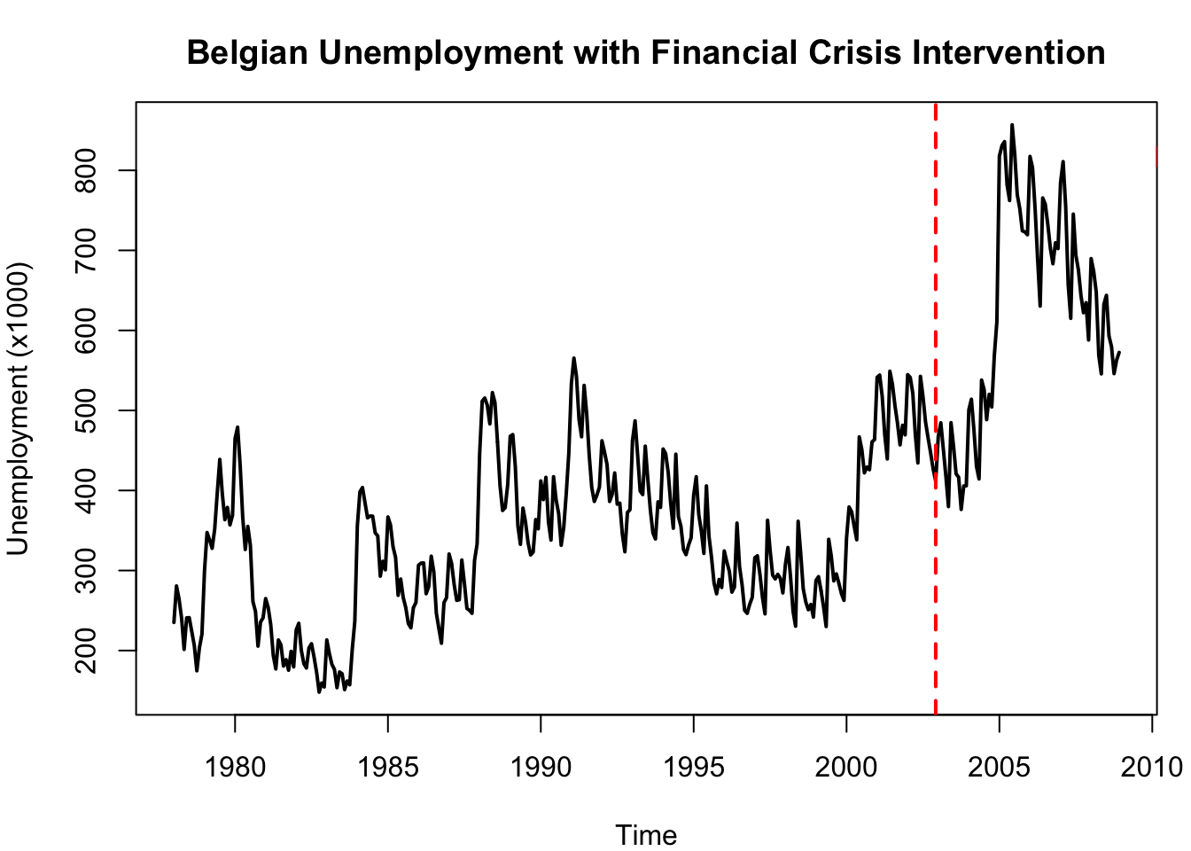
# Step intervention at the financial crisis (around observation 300, late 2008)
T_crisis <- 300
step_crisis <- c(rep(0, T_crisis - 1), rep(1, length(unemployment) - T_crisis + 1))

# Fit ARIMA with intervention (using same order as in estARIMA.qmd)
fit_unemp <- arima(sqrt(unemp_ts),
                   order = c(2, 1, 1),
                   seasonal = list(order = c(0, 1, 1), period = 12),
                   xreg = step_crisis)
cat("ARIMA(2,1,1)(0,1,1)[12] with financial crisis intervention:\n")
print(fit_unemp)

ARIMA(2,1,1)(0,1,1)[12] with financial crisis intervention:

Call:
arima(x = sqrt(unemp_ts), order = c(2, 1, 1), seasonal = list(order = c(0, 1, 
    1), period = 12), xreg = step_crisis)

Coefficients:
         ar1     ar2      ma1     sma1  step_crisis
      0.4577  0.1919  -0.3770  -0.7209      -0.2703
s.e.  0.1705  0.0653   0.1716   0.0404       0.4842

sigma^2 estimated as 0.2823:  log likelihood = -286.85,  aic = 585.71

par(mar = c(4, 4, 3, 1))
plot(unemp_ts, lwd = 2, ylab = "Unemployment (x1000)",
     main = "Belgian Unemployment with Financial Crisis Intervention")
abline(v = 1978 + (T_crisis - 1) / 12, col = "red", lwd = 2, lty = 2)
text(2009.5, max(unemployment) * 0.95, "Financial crisis", col = "red", pos = 4)

Figure 154.5: Unemployment: effect of the 2008 financial crisis intervention

The intervention captures the structural break that differencing alone cannot fully account for.

154.7 If Intervention Timing Is Unknown

The chapter examples assume that intervention timing is known from domain context (policy date, war event, regulation date). When timing is uncertain, a defensible workflow is:

1. Use domain knowledge to define a plausible date window.
2. Run structural break diagnostics (e.g. supF/CUSUM/Bai-Perron breakpoints) as candidate generators.
3. Test a small set of intervention dates and forms (pulse vs step, abrupt vs gradual).
4. Keep the specification that remains interpretable and passes residual diagnostics.

In R, strucchange::breakpoints() can be used to suggest candidate break dates before fitting the intervention ARIMA model.

154.8 Multiple Interventions

Real time series often experience more than one exceptional event. The intervention model extends naturally to multiple events:

\[ Y_t = v_1(B) I_{1,t}^{(T_1)} + v_2(B) I_{2,t}^{(T_2)} + \ldots + N_t \]

In R, this simply means adding multiple columns to the xreg matrix. Each column represents one intervention variable.

As an example, the Seatbelts series experienced both the 1973 oil crisis (which reduced driving and therefore casualties) and the 1983 seatbelt law. We can model both events simultaneously.

# Seatbelts: two interventions
data(Seatbelts)
y <- Seatbelts[, "DriversKilled"]
y_ts <- ts(y, start = c(1969, 1), frequency = 12)
n <- length(y)

# Oil crisis: step at January 1974 (observation 61)
step_oil <- c(rep(0, 60), rep(1, n - 60))
# Seatbelt law: step at January 1983 (observation 169)
step_law <- c(rep(0, 168), rep(1, n - 168))

xreg_both <- cbind(oil_crisis = step_oil, seatbelt_law = step_law)

fit_both <- arima(y_ts,
                  order = c(1, 0, 0),
                  seasonal = list(order = c(1, 1, 1), period = 12),
                  xreg = xreg_both)
cat("ARIMA with two interventions:\n")
print(fit_both)
cat("\nEstimated effects:\n")
cat("  Oil crisis effect:", round(coef(fit_both)["oil_crisis"], 1),
    "drivers killed/month\n")
cat("  Seatbelt law effect:", round(coef(fit_both)["seatbelt_law"], 1),
    "drivers killed/month\n")

ARIMA with two interventions:

Call:
arima(x = y_ts, order = c(1, 0, 0), seasonal = list(order = c(1, 1, 1), period = 12), 
    xreg = xreg_both)

Coefficients:
         ar1    sar1     sma1  oil_crisis  seatbelt_law
      0.3299  0.1710  -1.0000    -13.7251      -18.8832
s.e.  0.0719  0.0811   0.1747      4.1068        5.3280

sigma^2 estimated as 224.5:  log likelihood = -757.43,  aic = 1526.86

Estimated effects:
  Oil crisis effect: -13.7 drivers killed/month
  Seatbelt law effect: -18.9 drivers killed/month

154.9 Purpose, Pros & Cons

Purpose: Intervention analysis allows the analyst to account for known external events that cause structural breaks in a time series. It extends the pure ARIMA model to handle situations where the ceteris paribus assumption is violated.

Advantages:

• Formally incorporates domain knowledge about known events
• Improves both the fit and the forecasting accuracy of ARIMA models
• Provides estimates of the event’s effect (magnitude and significance)
• Uses the same estimation framework as standard ARIMA (arima() with xreg)

Limitations:

• The intervention must be a known event — the analyst must specify when it occurred
• The form of the intervention (pulse, step, gradual) must be chosen a priori
• If the event timing is unknown, other methods (e.g. structural break detection) are needed
• The input variable is binary — for continuous external variables, the Transfer Function model (Chapter 156) is needed

154.10 Tasks

1. Fit the Seatbelts model with a pulse for a single anomalous month (e.g. a month with an unusual spike in casualties) instead of a step. How does the model change compared to the step intervention?

2. Add a second intervention to the Soldiers model. For instance, consider the “surge” of troops in early 2007 (around observation 46) as an additional event. Does the model improve?

3. The tsplot app (Chapter 146) provides ARIMA forecasts. Load the Unemployment data and compare a pure ARIMA forecast (without intervention) to the intervention model from this chapter. Which forecast is more accurate for the post-crisis period?

Box, George E. P., and George C. Tiao. 1975. “Intervention Analysis with Applications to Economic and Environmental Problems.” Journal of the American Statistical Association 70 (349): 70–79. https://doi.org/10.1080/01621459.1975.10480264.