The Dirichlet distribution is the multivariate generalization of the Beta distribution. It is a probability distribution over the \((K-1)\)-simplex — the set of \(K\)-dimensional vectors whose components are non-negative and sum to one. The Dirichlet distribution arises naturally as the conjugate prior for the Multinomial distribution in Bayesian inference.
Formally, a random vector \(\mathbf{X} = (X_1, \ldots, X_K)\) is said to follow a Dirichlet distribution (i.e. \(\mathbf{X} \sim \text{Dir}(\boldsymbol{\alpha})\)) with concentration parameters \(\alpha_1, \ldots, \alpha_K > 0\) if the components satisfy \(X_i \geq 0\) and \(\sum_{i=1}^K X_i = 1\).
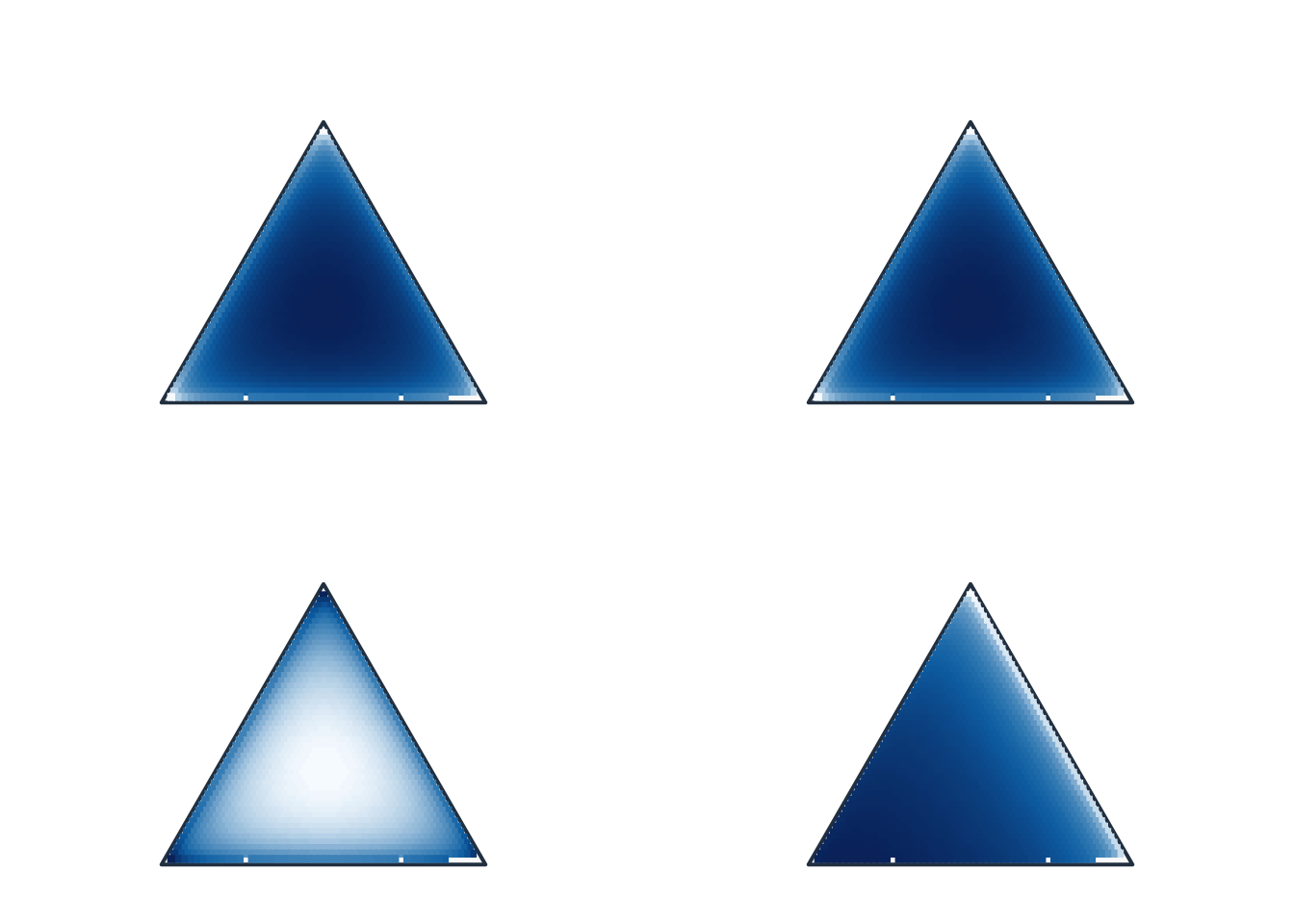
When any \(\alpha_i \leq 1\), the density concentrates at simplex boundaries (corners or edges) and the mode lies on the boundary of the simplex.
44.8 Parameter Estimation
The maximum likelihood estimators for \(\boldsymbol{\alpha}\) have no closed form and require iterative methods (e.g., Newton-Raphson on the log-likelihood). A method-of-moments estimator uses:
A market analyst models the share of three brands using a Dirichlet prior with \(\boldsymbol{\alpha} = (3, 5, 2)\). After observing 30 purchases with counts \((12, 14, 4)\), the posterior is \(\text{Dir}(15, 19, 6)\).
Merging categories preserves the Dirichlet: if \(\mathbf{X} \sim \text{Dir}(\alpha_1, \ldots, \alpha_K)\) and we define \(Y = X_1 + X_2\), then \((Y, X_3, \ldots, X_K) \sim \text{Dir}(\alpha_1 + \alpha_2, \alpha_3, \ldots, \alpha_K)\).
44.13 Property 3: Conjugate Prior for Multinomial
If \(\boldsymbol{\theta} \sim \text{Dir}(\boldsymbol{\alpha})\) is the prior on category probabilities and \(\mathbf{n} = (n_1, \ldots, n_K)\) are observed multinomial counts, then the posterior is: