A conditional inference tree is a non-parametric classification and regression method that uses a statistical testing framework to select variables and determine split points. Unlike traditional decision trees (CART; Breiman et al. (1984)), conditional inference trees use permutation tests to evaluate the association between each predictor and the response variable, avoiding the variable selection bias that occurs with greedy algorithms.
The method was introduced by Hothorn, Hornik, and Zeileis (Hothorn, Hornik, and Zeileis (2006)) and is implemented in the party package in R via the ctree() function.
140.2 Algorithm
The algorithm proceeds as follows:
Test for independence: For each predictor variable, test the null hypothesis of independence between the predictor and the response using permutation tests based on the conditional distribution of linear statistics.
Variable selection: Select the predictor with the strongest association to the response (smallest p-value). If the smallest p-value is above the significance threshold, stop splitting.
Split point selection: For the selected predictor, find the split point that maximizes a two-sample statistic.
Recursion: Repeat the process for each child node until a stopping criterion is met.
140.3 Statistical Testing Framework
The key difference from traditional decision trees is the use of conditional inference. For each predictor \(X_j\), the algorithm computes a test statistic based on influence functions and a linear statistic:
\(g_j\) is a transformation of the predictor (e.g., indicator functions for factors)
\(h\) is an influence function for the response
The p-value is computed using the permutation distribution of this statistic, conditional on the observed data.
140.4 Control Parameters
The ctree_control() function specifies the stopping criteria:
Table 140.1: Control parameters for conditional inference trees
Parameter
Description
Default
mincriterion
1 - p-value threshold for splitting
0.95
minsplit
Minimum observations for attempting a split
20
minbucket
Minimum observations in terminal nodes
7
maxdepth
Maximum tree depth
Inf
A higher mincriterion requires stronger evidence to split (more conservative tree). Setting mincriterion = 0.95 corresponds to a significance level of \(\alpha = 0.05\).
140.5 Comparison with CART
Table 140.2: Comparison of CART and Conditional Inference Trees
Aspect
CART
Conditional Inference Tree
Variable selection
Greedy (maximizes impurity reduction)
Statistical testing
Selection bias
Favors variables with many splits
Unbiased
Pruning
Required (post-hoc)
Built-in via significance testing
Split criterion
Gini, entropy, or variance
Permutation test p-values
Interpretability
High
High
140.6 R Module
140.6.1 Public website
Conditional Inference Trees are available on the public website:
The Conditional Inference Tree module is available in RFC under the menu “Models / Conditional Inference Tree”.
An interactive model-building application that includes conditional inference trees alongside other classification methods (logistic regression, naive Bayes, conditional forests) is available under “Models / Manual Model Building”. In its Tree tab, binary classification trees expose a classification threshold. That threshold converts predicted probabilities into predicted classes, so changing it changes the confusion matrix, sensitivity, specificity, and precision. This application therefore lets users compare model performance using ROC curves (Chapter 60) and confusion matrices (Chapter 59).
140.6.3 R Code
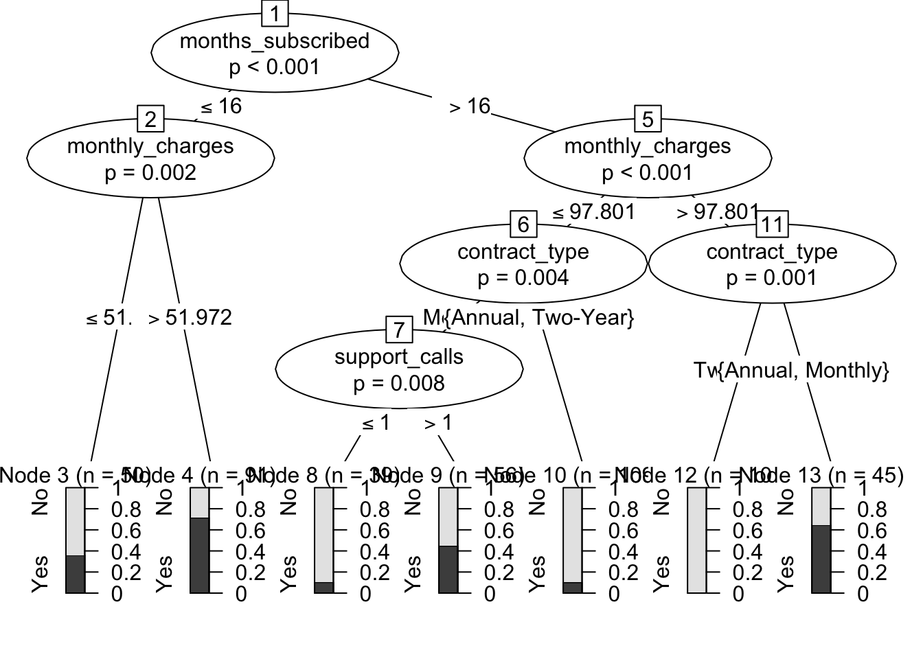
The following code demonstrates fitting a conditional inference tree for classification:
Figure 140.1: Conditional inference tree for classification
140.7 Predictions
Predictions from a conditional inference tree include both class predictions and class probabilities:
# Class predictionshead(predict(tree))# Class probabilitiesprobs <-do.call(rbind, treeresponse(tree))colnames(probs) <-levels(df$churn)head(probs)
[1] Yes No  No  No  No  No
Levels: No Yes
            No       Yes
[1,] 0.2857143 0.7142857
[2,] 0.8990826 0.1009174
[3,] 0.8974359 0.1025641
[4,] 0.8990826 0.1009174
[5,] 0.8990826 0.1009174
[6,] 0.8990826 0.1009174
The predicted probabilities can be used for ROC analysis (Chapter 60) to evaluate classifier performance and determine optimal classification thresholds.
140.8 Example: Medical Diagnosis
A hospital wants to predict disease presence based on patient characteristics:
      Predicted
Actual  No Yes
   No  103   7
   Yes  38  32
[1] 0.75
Code
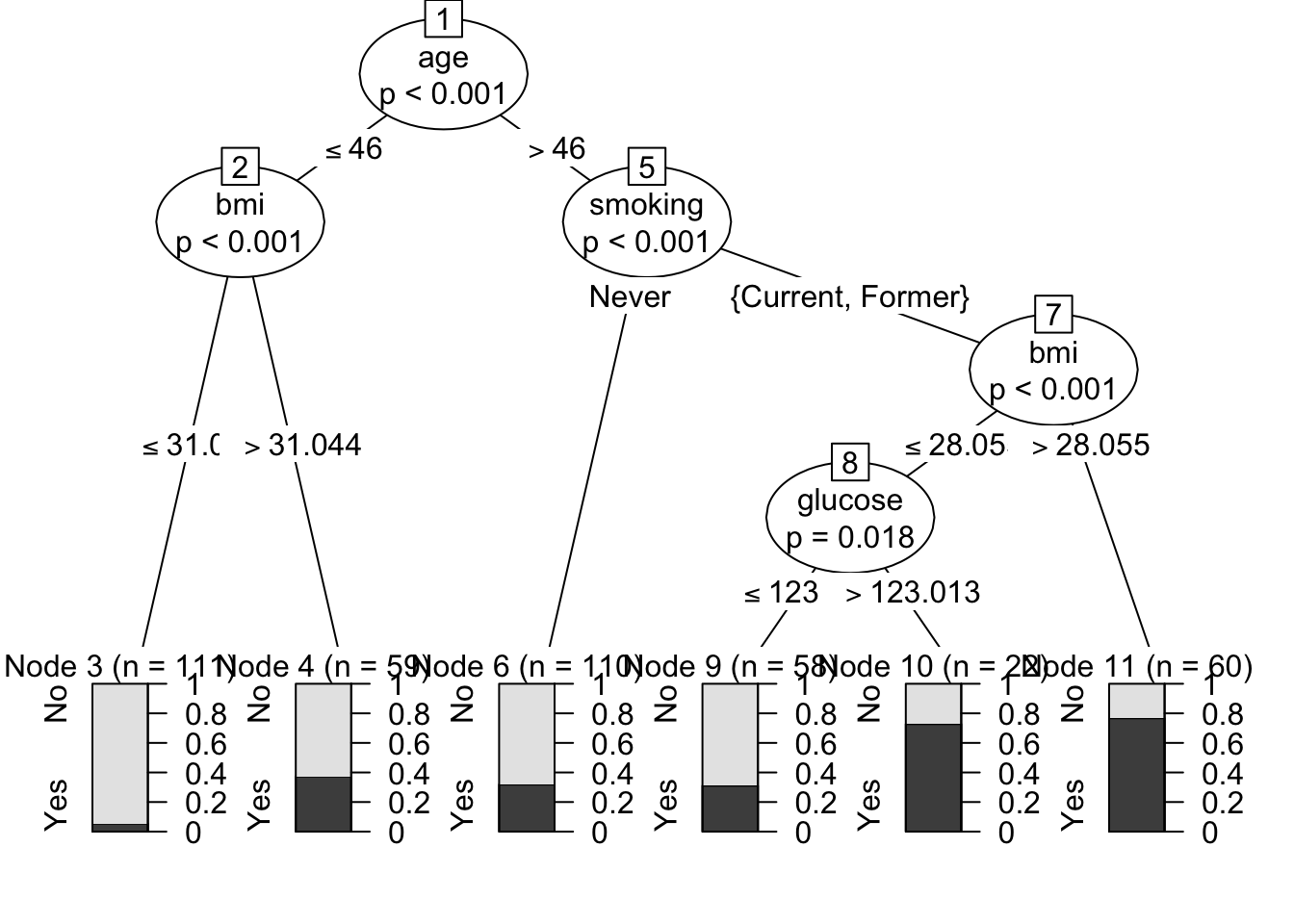
plot(disease_tree)
Figure 140.2: Conditional inference tree for disease prediction
140.9 Classification Thresholds for Binary Trees
For a binary outcome, the tree does not only produce a class label. It first produces a probability for the positive class. The final class label is obtained by comparing that probability with a threshold.
Using a threshold of 0.50 means that the model predicts Yes only when the estimated probability of disease is at least 50%. Lowering the threshold makes positive predictions easier to trigger. That usually increases sensitivity but may reduce specificity and precision.
Changing the threshold changes the binary tree’s classification behavior
Threshold
Accuracy
Sensitivity
Specificity
Precision
0.50
0.75
0.457
0.936
0.821
0.35
0.75
0.557
0.873
0.736
This is the same logic used in the Tree tab of Models / Manual Model Building: the fitted tree supplies class probabilities, and the threshold determines where the final yes/no boundary is drawn.
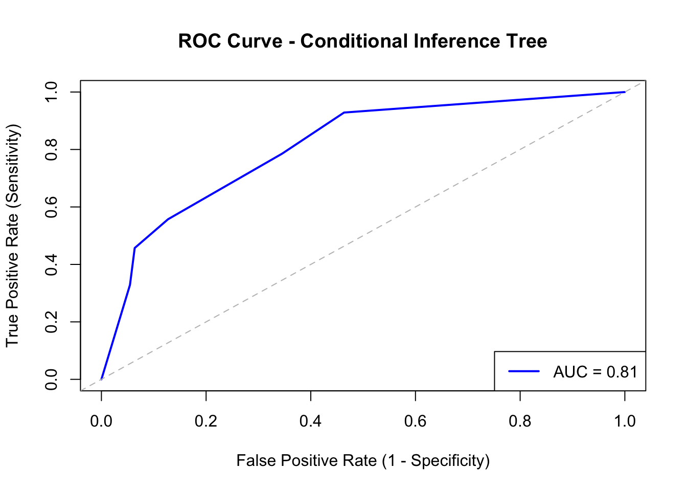
140.10 ROC Analysis Integration
The predicted probabilities from a conditional inference tree can be used to construct ROC curves (Chapter 60) for evaluating and comparing classifier performance:
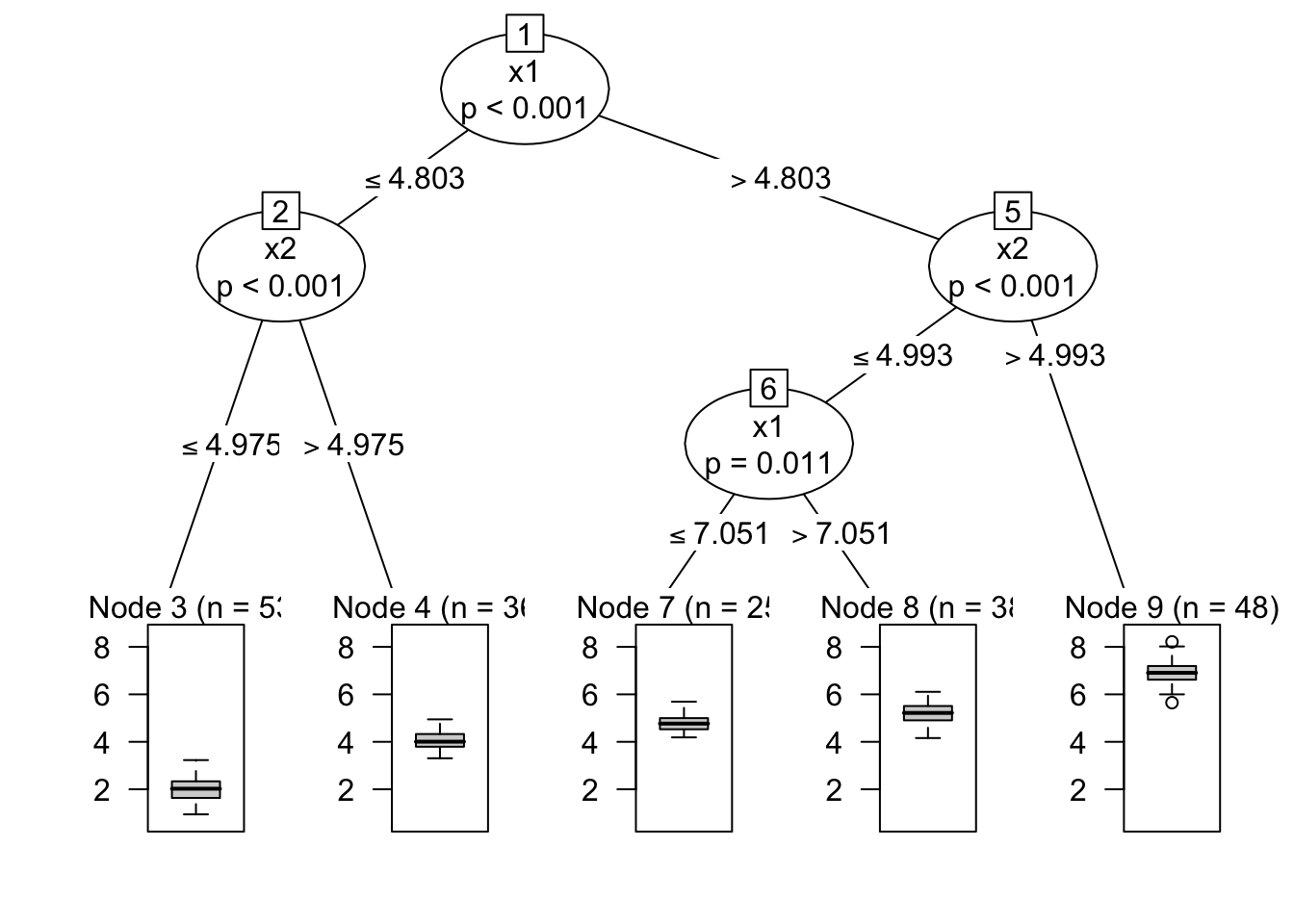
Figure 140.4: Conditional inference tree for regression
When the outcome is continuous, the tree plot itself is only the first diagnostic layer. The next question is whether the terminal nodes are equally reliable. Some leaves can have tight, well-behaved outcome distributions, whereas others can have broad spread or strong skewness even if their fitted mean looks usable. The follow-up chapter on leaf-wise distribution checks, Chapter 141, shows how to inspect that uncertainty inside the fitted terminal nodes rather than stopping at the tree diagram.
140.12 Variable Importance
While conditional inference trees do not have a built-in variable importance measure like random forests, the variables that appear higher in the tree (closer to the root) are generally more important. The number of times a variable is used for splitting across the tree can also indicate importance. If you need a model class that formalizes importance through an ensemble rather than a single diagram, the next chapter on Chapter 142 is the natural continuation.
140.13 Pros & Cons
140.13.1 Pros
Conditional inference trees have the following advantages:
Unbiased variable selection due to statistical testing framework.
No need for post-hoc pruning; tree size is controlled by significance threshold.
Handles mixed predictor types (numeric and categorical) naturally.
Provides interpretable decision rules.
Less prone to overfitting compared to CART when using appropriate mincriterion.
140.13.2 Cons
Conditional inference trees have the following disadvantages:
Computationally more intensive than CART due to permutation tests.
May produce smaller trees than CART, potentially underfitting in some cases.
The permutation test framework assumes exchangeability under the null hypothesis.
Variable importance is less straightforward than in ensemble methods.
A single fitted tree can be unstable if the training sample changes; Chapter 142 shows how ensembling is used to reduce that instability when prediction matters more than a single interpretable diagram.
Cannot extrapolate beyond the range of training data.
140.14 Task
Using the iris dataset, fit a conditional inference tree to classify species based on sepal and petal measurements. Visualize the tree and interpret the decision rules.
Compare the performance of a conditional inference tree with logistic regression (Chapter 136) on a binary classification problem. Use ROC curves and AUC (Section 60.4) to evaluate both models.
Experiment with different values of mincriterion (0.90, 0.95, 0.99) and observe how tree complexity changes. Discuss the trade-off between tree size and prediction accuracy.
Fit a regression tree to predict mpg in the mtcars dataset. Compare the predictions with those from a linear regression model (Chapter 134).
Breiman, Leo, Jerome H. Friedman, Richard A. Olshen, and Charles J. Stone. 1984. Classification and Regression Trees. Belmont, CA: Wadsworth International Group.
Hothorn, T., K. Hornik, and A. Zeileis. 2006. “Unbiased Recursive Partitioning: A Conditional Inference Framework.”Journal of Computational and Graphical Statistics 15: 651–74.